Template:OceanMesh UGrid from Coverage Tool: Difference between revisions
No edit summary |
|||
| (19 intermediate revisions by the same user not shown) | |||
| Line 4: | Line 4: | ||
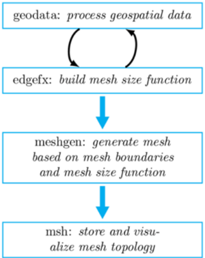
The ''OceanMesh UGrid from Coverage'' tool is used to create an unstructured triangular mesh from either a map coverage or a vector file on disk containing shoreline features. The algorithms from OceanMesh2D (https://github.com/CHLNDDEV/OceanMesh2D, Roberts et al. 2019) are used to process the coverage, building mesh sizing functions, and produce a mesh that is valid for numerical simulation (Figure 1). | The ''OceanMesh UGrid from Coverage'' tool is used to create an unstructured triangular mesh from either a map coverage or a vector file on disk containing shoreline features. The algorithms from OceanMesh2D (https://github.com/CHLNDDEV/OceanMesh2D, Roberts et al. 2019) are used to process the coverage, building mesh sizing functions, and produce a mesh that is valid for numerical simulation (Figure 1). | ||
[[File:OceanMesh2D Workflow.png|thumb|none| | :[[File:OceanMesh2D Workflow.png|thumb|none|300 px|Figure 1: Typical workflow in OceanMesh2D from Roberts et al. (2019) that has been adapted into SMS as a callable plugin. ]] | ||
The process to build a mesh using the OceanMesh2D program historically involved writing a MATLAB or Python script following the overall approach indicated in Figure 1 looping over vector and raster data to build sizing functions and then using the sizing function to build an unstructured mesh with the provided API call. Now with this plugin, the user can graphically specify their inputs and parameters without writing a Python or MATLAB script. In addition, the mesh becomes directly editable inside the SMS GUI after generation. | The process to build a mesh using the OceanMesh2D program historically involved writing a MATLAB or Python script following the overall approach indicated in Figure 1 looping over vector and raster data to build sizing functions and then using the sizing function to build an unstructured mesh with the provided API call. Now with this plugin, the user can graphically specify their inputs and parameters without writing a Python or MATLAB script. In addition, the mesh becomes directly editable inside the SMS GUI after generation. | ||
With this plugin, similar to the MATLAB and Python versions of OceanMesh2D, the user has the option to configure the mesh resolution throughout the domain with several mesh sizing heuristics based on the information contained within the map coverage and a topobathymetric raster objectively according to size function heuristics. | With this plugin, similar to the MATLAB and Python versions of OceanMesh2D, the user has the option to configure the mesh resolution throughout the domain with several mesh sizing heuristics based on the information contained within the map coverage and a topobathymetric raster objectively according to size function heuristics. | ||
In the OceanMesh2D approach, the domain to-be-meshed is the intersection area between a user-specified polygon and the multiple polygons contained in a shoreline coverage (Figure 2). This implies that all inputs to OceanMesh2D must be provided as polygons orientated in the correct way, so the intersection area between them defines the intended area to be meshed. | |||
[[File:OceanMesh2D domain to-be-meshed.png|thumb|none|400 px| Figure 2: The area to-be-meshed is represented as a blue hatched region and is the intersection area between the red and green polygons that represent the shoreline. The black-dashed polygon represents the model domain. The “inner” category represents polygons fully enclosed in the meshing domain while the “mainland” polygons are partially enclosed in the meshing domain.]] | |||
====Inputs==== | ====Inputs==== | ||
*''Shoreline Coverage with polygons (optional)'' – Select a map coverage that contains shoreline features as polygons. Note the coverages must be composed of only polygons and a map projection must be set. Note that this is a required argument if “Input shoreline coverage as a vector file” is not specified. | <!--*''Shoreline Coverage with polygons (optional)'' – Select a map coverage that contains shoreline features as polygons. Note the coverages must be composed of only polygons and a map projection must be set. Note that this is a required argument if “Input shoreline coverage as a vector file” is not specified.--> | ||
*''Modify options to simplify polygons (optional)'' – By default all polygons part of the shoreline coverage are “simplified” | *''Specify inputs from coverage or vector file'' – Specify the input polygons representing the shoreline to be input to plugin. Either the user specifies a map coverage that is open in SMS or they specify the path to a vector file that’s on disk. Note that in both cases the map coverage must be composed of only polygons that are topologically valid. This means they do to contain self-intersections and other types of degenerate geometries. Both input option types require the Coordinate Reference System (CRS) to be specified as well and if not, an error message will display. | ||
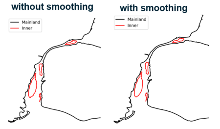
*''Modify options to simplify polygons (optional)'' – By default all polygons part of the shoreline coverage are “simplified” using a moving window smoothing approach. In other words, after resampling the shorelineto an equal spacing between adjacent nodes, a window is centered on a given node and the average coordinate of all the nodes in the window replaces the value of the selected node. This helps to filter relatively small-scale features along the shoreline polygons that may not be impactful for coastal modelling applications. A larger odd integer value selected (3 by default) for the “Smoothing Window” will produce smoother shoreline boundaries. Care however must be taken to ensure acceptable distortion of the shoreline coverage through the application of the moving average smoothing (Figure 3). | |||
*: [[File:OceanMesh2D shoreline smoothing.png|thumb|none|450 px|Figure 3: Illustrates the shoreline smoothing functionality that can be enabled/disabled. Care must be taken when using this option to avoid too much distortion in the representation of the shoreline.]] | |||
*''Area Threshold Multiplier'' – Polygons with an area less than “Area Threshold Multiplier” x “Minimum Mesh Size”^2 are removed from the input coverage. These small polygons are likely to be difficult to represent at the given “Minimum Mesh Size” scale and may cause simulation challenges. | *''Area Threshold Multiplier'' – Polygons with an area less than “Area Threshold Multiplier” x “Minimum Mesh Size”^2 are removed from the input coverage. These small polygons are likely to be difficult to represent at the given “Minimum Mesh Size” scale and may cause simulation challenges. | ||
*''Input shoreline coverage as a vector file (optional)'' – In the case a map coverage is not loaded, the user can select a vector file (i.e., ESRI Shapefile or geopackage) on disk with only polygons and a specified map projection. This is a required if ''Shoreline Coverage with polygons'' is not specified. | <!--*''Input shoreline coverage as a vector file (optional)'' – In the case a map coverage is not loaded, the user can select a vector file (i.e., ESRI Shapefile or geopackage) on disk with only polygons and a specified map projection. This is a required if ''Shoreline Coverage with polygons'' is not specified. | ||
** Options: Options are shared with those described under “Shoreline Coverage with polygons (optional)” (c.f., “Modify options to simplify polygons”). | ** Options: Options are shared with those described under “Shoreline Coverage with polygons (optional)” (c.f., “Modify options to simplify polygons”).--> | ||
*''Domain coverage as a polygon'' – Select a map coverage from the loaded coverages that represents the area to-be-meshed (i.e., the domain) as a single polygon. Note that the area to-be-meshed is the waterside portion of the intersection area between the shoreline polygons and the domain polygon. | *''Domain coverage as a polygon'' – Select a map coverage from the loaded coverages that represents the area to-be-meshed (i.e., the domain) as a single polygon. Note that the area to-be-meshed is the waterside portion of the intersection area between the shoreline polygons and the domain polygon. | ||
*''Invert the area to-be-meshed (optional)'' – this option inverts the meshing domain from the existing configuration. | *''Invert the area to-be-meshed (optional)'' – this option inverts the meshing domain from the existing configuration. | ||
** '''''When to use:''''' When meshing lakes and sections of rivers that are not connected to the open ocean, the area meshed may be inverted. For instance, the landside of the domain will be meshed instead of the desired oceanside portion. In this case, this option should be enabled. | ** '''''When to use:''''' When meshing lakes and sections of rivers that are not connected to the open ocean, the area meshed may be inverted. For instance, the landside of the domain will be meshed instead of the desired oceanside portion. In this case, this option should be enabled. | ||
*''Minimum mesh size'' – | Mesh size is measured on a per element basis and represents the minimum edge length of a triangular element. In the ideal case all elements are equilateral, then all edge lengths should be equal. Size constraints are bonded in the mesh sizing function. | ||
*''Maximum mesh size'' – | *''Minimum mesh size'' – The approximate desired minimum mesh size used throughout the domain in the units of the map projection. Note in the case of geographic inputs, the size argument will be converted into equatorial degrees. | ||
*''Rate of change in mesh size'' – | *''Maximum mesh size'' – The approximate desired maximum mesh size used throughout the domain in the units of the map projection. Note in the case of geographic inputs, the size argument will be converted into equatorial degrees. | ||
*''Rate of change in mesh size'' – The approximate rate of change in mesh sizes. Mesh size change is measured as the ratio of the average triangular edge length between adjacent triangles. Note that the mesh sizing function is gradient limited using the approach (Persson 2004) not the unstructured mesh and as a result, the limiting is approximate. | |||
The following options below are used to control the variability of mesh sizing in the domain. | The following options below are used to control the variability of mesh sizing in the domain. | ||
| Line 28: | Line 34: | ||
** Distance-sizing: elemental resolution is a minimum along the shoreline and expands linearly in size at the specified “Rate of change in mesh size”. | ** Distance-sizing: elemental resolution is a minimum along the shoreline and expands linearly in size at the specified “Rate of change in mesh size”. | ||
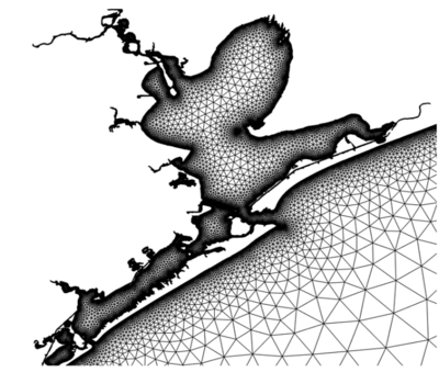
*** '''''When to use:''''' This heuristic can be useful for building meshes for relatively small regions like a harbor, small estuary, or bay in which the modeler can computationally afford to place the minimum resolution along the entire extent of the shoreline everywhere. | *** '''''When to use:''''' This heuristic can be useful for building meshes for relatively small regions like a harbor, small estuary, or bay in which the modeler can computationally afford to place the minimum resolution along the entire extent of the shoreline everywhere. | ||
*:[[File:OceanMesh2D distance sizing.png|thumb|none|400 px|Figure 4: Example of a mesh with elements using the distance sizing approach.]] | |||
** Feature-sizing: elemental resolution is placed according to the shoreline “thickness” or “width” with the user-specified number of elements placed across the calculated shoreline “width”. Shoreline “thickness” or “width” is computed through the medial axis transform of the specified shoreline coverage. | ** Feature-sizing: elemental resolution is placed according to the shoreline “thickness” or “width” with the user-specified number of elements placed across the calculated shoreline “width”. Shoreline “thickness” or “width” is computed through the medial axis transform of the specified shoreline coverage. | ||
*** Options: | *** Options: | ||
**** Number of elements per shoreline width: | **** ''Number of elements per shoreline width:'' This number of triangular elements will be placed across the width of the shoreline. For example, if there is an inlet that is 100-m wide and the specified value for this parameter is 3, then three ~33-m elements would be placed in this region. Note however the minimum element size is globally bounded by the “Minimum mesh size” parameter. | ||
**** ''Maximum element size nearshore:'' At distances less than the ''Distance from the shoreline used to apply the maximum element size nearshore'' this from the shoreline, the mesh resolution is bounded. If left un-specified, mesh resolution can grow to the specified “Maximum mesh size” nearshore undesirable for certain modelling applications. Note units must follow the map projection. | |||
**** Maximum element size nearshore: | **** ''Distance from shoreline used to apply the maximum element size nearshore:'' At distances less than this from the shoreline, the “Maximum element size nearshore” is enforced. Note units must follow the map projection. | ||
**** Distance from shoreline used to apply the maximum element size nearshore: | |||
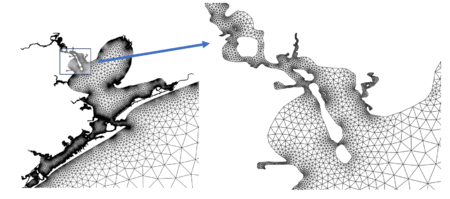
** '''''When to use:''''' Useful for building meshes for relatively larger domains where the user needs to economize on the total model size (in terms of number of degrees-of-freedom/nodes). This heuristic will relax mesh resolution in areas that are geometrically “simple” (e.g., straight) and refine mesh resolution in areas that are more complex (curvier). | ** '''''When to use:''''' Useful for building meshes for relatively larger domains where the user needs to economize on the total model size (in terms of number of degrees-of-freedom/nodes). This heuristic will relax mesh resolution in areas that are geometrically “simple” (e.g., straight) and refine mesh resolution in areas that are more complex (curvier). | ||
*: [[File:OceanMesh2D feature sizing.png|thumb|none|450 px|Figure 5: Example of a mesh with elements using the feature-sizing approach. ]] | |||
*''Mesh sizing function #2 (optional):'' | *''Mesh sizing function #2 (optional):'' | ||
**''Wavelength-to-gridscale:'' | **''Wavelength-to-gridscale:'' The local wavelength of a shallow-water wave with user-specified period is calculated (by default the period of the M2 semi-diurnal tidal constituent 12.42 hours is specified) and gravity is assumed to be 9.81 m/s^2. Elemental resolution is then determined by dividing the calculated wavelength by the “Number of elements per wavelength” parameter (by default 100). This sizing function requires a digital elevation model be specified via “Input DEM for select mesh sizing functions” option. | ||
***Options: | ***Options: | ||
****“Number of elements per wavelength” used to divide the estimated shallow water wavelength to produce the local mesh resolution. | ****“Number of elements per wavelength” used to divide the estimated shallow water wavelength to produce the local mesh resolution. | ||
****“Period of wave (seconds)” used to compute the wavelength. | ****“Period of wave (seconds)” used to compute the wavelength. | ||
***'''''When to use:''''' For regional modelling applications, it is important to distribute enough number of nodes in continental shelf regions to represent the processes that generate storm surge. A key benefit of this heuristic is smooth mesh sizing transitions that vary proportional to the square root of the water depth. For storm surge modelling applications, it can be useful to combine this mesh sizing function with “Mesh Sizing Function #1” to ensure mesh resolution does not grow too large on large and shallow continental shelves. | ***'''''When to use:''''' For regional modelling applications, it is important to distribute enough number of nodes in continental shelf regions to represent the processes that generate storm surge. A key benefit of this heuristic is smooth mesh sizing transitions that vary proportional to the square root of the water depth. For storm surge modelling applications, it can be useful to combine this mesh sizing function with “Mesh Sizing Function #1” to ensure mesh resolution does not grow too large on large and shallow continental shelves (Figure 6). | ||
*:[[File:OceanMesh2D distance-sizing wavelength.png|thumb|none|450 px|Figure 6: Comparison between a mesh generated solely using a distance-sizing function (left panel) and a mesh incorporating both distance and wavelength sizing functions (right panel). This example illustrates the element distribution according to a wavelength-to-grid scale mesh sizing function. The parameter "Number of elements per wavelength" enhances resolution on the continental shelf.]] | |||
*Mesh sizing function #3 (optional): | *Mesh sizing function #3 (optional): | ||
**''CFL Timestep Bounding:'' This mesh sizing function adjusts the mesh sizing function so an estimated upper bound of the Courant number is respected, assuming a user-specified simulation | **''CFL Timestep Bounding:'' This mesh sizing function adjusts the mesh sizing function so an estimated upper bound of the Courant number is respected, assuming a user-specified simulation time step. Note this function does not act to refine the mesh in the case that a minimum Courant number is necessary, which is common in ALE schemes for example used by SCHISM. This will be incorporated in later developments. | ||
***'''''When to use:''''' It is generally always encouraged to incorporate this sizing function when | ***'''''When to use:''''' It is generally always encouraged to incorporate this sizing function when there is topobathymetryic data that intended to interpolate onto the mesh nodes. This encourages the numerical stability of the developed model when simulation is attempted. The Courant number is estimated through the canonical approach as the ratio of user-specified simulation time step in seconds multiplied by the shallow-water wave speed in meters per second divided by the local mesh resolution in meters. This sizing function requires a digital elevation model be specified via “Input DEM for select mesh sizing functions” option. | ||
***Options: | ***Options: | ||
****“Maximum Allowable Timestep (seconds)” - | ****“Maximum Allowable Timestep (seconds)” - The anticipated simulation time step. | ||
****“Maximum Allowable Courant Number for given timestep” – | ****“Maximum Allowable Courant Number for given timestep” – The upper bound Courant number that will violate the CFL condition of the numerical scheme. | ||
*:The tool constructs each sizing function independently, then computes their spatial minimum to synthesize the "final mesh sizing function." | *:The tool constructs each sizing function independently, then computes their spatial minimum to synthesize the "final mesh sizing function." | ||
*''Filename of mesh sizing function'' – the final mesh sizing function used to generate the mesh is exported as a geotiff. Note this file will automatically visualize after execution of the tool inside SMS. | *''Filename of mesh sizing function'' – the final mesh sizing function used to generate the mesh is exported as a geotiff. Note this file will automatically visualize after execution of the tool inside SMS. | ||
| Line 54: | Line 61: | ||
***“Minimum boundary quality” – All boundary elements with a mesh quality () less than this threshold will be deleted. | ***“Minimum boundary quality” – All boundary elements with a mesh quality () less than this threshold will be deleted. | ||
***“Disconnected areas with this percent of the total area are removed” – Portions of the mesh that are disconnected with an area less than this percent of the total mesh will be deleted. For example, removing disconnected inland lakes when meshing a coastal domain. | ***“Disconnected areas with this percent of the total area are removed” – Portions of the mesh that are disconnected with an area less than this percent of the total mesh will be deleted. For example, removing disconnected inland lakes when meshing a coastal domain. | ||
***“Maximum number of iterations for Laplace smoothing” – | ***“Maximum number of iterations for Laplace smoothing” – The maximum number of iterations to apply Laplace smoothing. Move vertices to the average position of their connected neighbours. | ||
***“Minimum movement tolerance for Laplace smoothing” – | ***“Minimum movement tolerance for Laplace smoothing” – If an iteration of Laplace smoothing produces a nodal movement less than this tolerance, iterations will cease. | ||
*“Modify mesh generation options”: | *“Modify mesh generation options”: Users should only modify the following force functions if their mesh is not convergent and not producing a relatively high-quality discretization. In this case, it makes sense to increase the number of iterations 25 to 50% while lowering the pseudo timestep 25 to 50% and switching the force function to “person_strang” from the default “bossen_heckbert”. | ||
**Options: | **Options: | ||
***“Number of meshing iterations” | ***“Number of meshing iterations” – Number of meshing iterations to perform. Generally, more iterations imply a higher mesh quality at the cost of more time spent meshing. With that said almost all problems encountered saturate around 100 iterations. | ||
***“Pseudo timestep for meshing” – Mesh generation is solved using a force-balance approach (Roberts et al. 2019) that time marches the solution to a system of ordinary differential equations. Depending on the stiffness of the problem, the | ***“Pseudo timestep for meshing” – Mesh generation is solved using a force-balance approach (Roberts et al. 2019) that time marches the solution to a system of ordinary differential equations. Depending on the stiffness of the problem, the time step can be modified to achieve better results. Generally, if meshing is not convergent, then halving the time step is recommended. If meshing is converging rapidly in say less than 25 iterations, it may be possible to double the time step and achieve better resulrts. A suitable range is between 0.05 and 0.20 pseudo seconds. | ||
***Nodes are moved iteratively. Forces originate based on discrepancy between the edge lengths of the current triangulation and the mesh sizing function. | ***Nodes are moved iteratively. Forces originate based on discrepancy between the edge lengths of the current triangulation and the mesh sizing function. | ||
****“Force function used in mesh generation”. | ****“Force function used in mesh generation”. | ||
| Line 67: | Line 74: | ||
====Outputs==== | ====Outputs==== | ||
Name of the 2D triangular unstructured mesh that will be generated. A mesh will be visualized in the SMS GUI. | Name of the 2D triangular unstructured mesh that will be generated. A mesh will be visualized in the SMS GUI along with the sizing function as a contour filled image appearing behind the mesh. | ||
:[[File:OceanMesh2D mesh output example.png|thumb|none|450 px|Figure 7: Example of a developed mesh and the corresponding mesh sizing function used to be vary mesh resolution in the SMS GUI.]] | |||
====Current Location in Toolbox ==== | ====Current Location in Toolbox ==== | ||
Unstructured Grids/OceanMesh UGrid from Coverage | Unstructured Grids/OceanMesh UGrid from Coverage | ||
====References==== | ====References==== | ||
* Randolph E. Bank. PLTMG: A Software Package for Solving Elliptic Partial Differential Equations. Society for Industrial and Applied Mathematics, 1 1998. ISBN 978-0-89871-409-8. doi: 10.1137/ 1.9780898719635. URL [http://epubs.siam.org/doi/book/10.1137/1.9780898719635 http://epubs.siam.org/doi/book/10.1137/1.9780898719635]. | |||
* [https://github.com/CHLNDDEV/OceanMesh2D Ocean Mesh 2D on Github] | * [https://github.com/CHLNDDEV/OceanMesh2D Ocean Mesh 2D on Github] | ||
* Roberts, K. J., Pringle, W. J., and Westerink, J. J., 2019. OceanMesh2D 1.0: MATLAB-based software for two-dimensional unstructured mesh generation in coastal ocean modeling, Geosci. Model Dev. (GMD), [https://doi.org/10.5194/gmd-12-1847-2019]. | * Roberts, K. J., Pringle, W. J., and Westerink, J. J., 2019. OceanMesh2D 1.0: MATLAB-based software for two-dimensional unstructured mesh generation in coastal ocean modeling, Geosci. Model Dev. (GMD), [https://doi.org/10.5194/gmd-12-1847-2019 https://doi.org/10.5194/gmd-12-1847-2019]. | ||
* Persson, Per-Olof. "PDE-Based Gradient Limiting for Mesh Size Functions." IMR. 2004. | * Persson, Per-Olof. "PDE-Based Gradient Limiting for Mesh Size Functions." IMR. 2004. | ||
Latest revision as of 22:57, 1 July 2024
OceanMesh UGrid from Coverage
The OceanMesh UGrid from Coverage tool is used to create an unstructured triangular mesh from either a map coverage or a vector file on disk containing shoreline features. The algorithms from OceanMesh2D (https://github.com/CHLNDDEV/OceanMesh2D, Roberts et al. 2019) are used to process the coverage, building mesh sizing functions, and produce a mesh that is valid for numerical simulation (Figure 1).
The process to build a mesh using the OceanMesh2D program historically involved writing a MATLAB or Python script following the overall approach indicated in Figure 1 looping over vector and raster data to build sizing functions and then using the sizing function to build an unstructured mesh with the provided API call. Now with this plugin, the user can graphically specify their inputs and parameters without writing a Python or MATLAB script. In addition, the mesh becomes directly editable inside the SMS GUI after generation.
With this plugin, similar to the MATLAB and Python versions of OceanMesh2D, the user has the option to configure the mesh resolution throughout the domain with several mesh sizing heuristics based on the information contained within the map coverage and a topobathymetric raster objectively according to size function heuristics.
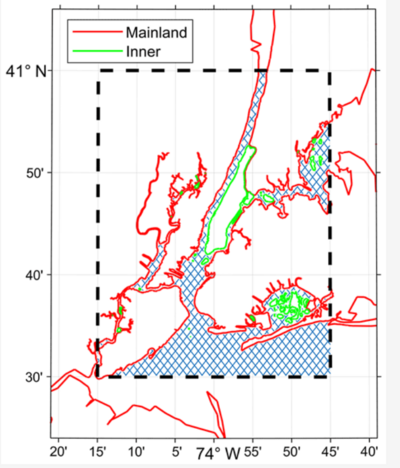
In the OceanMesh2D approach, the domain to-be-meshed is the intersection area between a user-specified polygon and the multiple polygons contained in a shoreline coverage (Figure 2). This implies that all inputs to OceanMesh2D must be provided as polygons orientated in the correct way, so the intersection area between them defines the intended area to be meshed.
Inputs
- Specify inputs from coverage or vector file – Specify the input polygons representing the shoreline to be input to plugin. Either the user specifies a map coverage that is open in SMS or they specify the path to a vector file that’s on disk. Note that in both cases the map coverage must be composed of only polygons that are topologically valid. This means they do to contain self-intersections and other types of degenerate geometries. Both input option types require the Coordinate Reference System (CRS) to be specified as well and if not, an error message will display.
- Modify options to simplify polygons (optional) – By default all polygons part of the shoreline coverage are “simplified” using a moving window smoothing approach. In other words, after resampling the shorelineto an equal spacing between adjacent nodes, a window is centered on a given node and the average coordinate of all the nodes in the window replaces the value of the selected node. This helps to filter relatively small-scale features along the shoreline polygons that may not be impactful for coastal modelling applications. A larger odd integer value selected (3 by default) for the “Smoothing Window” will produce smoother shoreline boundaries. Care however must be taken to ensure acceptable distortion of the shoreline coverage through the application of the moving average smoothing (Figure 3).
- Area Threshold Multiplier – Polygons with an area less than “Area Threshold Multiplier” x “Minimum Mesh Size”^2 are removed from the input coverage. These small polygons are likely to be difficult to represent at the given “Minimum Mesh Size” scale and may cause simulation challenges.
- Domain coverage as a polygon – Select a map coverage from the loaded coverages that represents the area to-be-meshed (i.e., the domain) as a single polygon. Note that the area to-be-meshed is the waterside portion of the intersection area between the shoreline polygons and the domain polygon.
- Invert the area to-be-meshed (optional) – this option inverts the meshing domain from the existing configuration.
- When to use: When meshing lakes and sections of rivers that are not connected to the open ocean, the area meshed may be inverted. For instance, the landside of the domain will be meshed instead of the desired oceanside portion. In this case, this option should be enabled.
Mesh size is measured on a per element basis and represents the minimum edge length of a triangular element. In the ideal case all elements are equilateral, then all edge lengths should be equal. Size constraints are bonded in the mesh sizing function.
- Minimum mesh size – The approximate desired minimum mesh size used throughout the domain in the units of the map projection. Note in the case of geographic inputs, the size argument will be converted into equatorial degrees.
- Maximum mesh size – The approximate desired maximum mesh size used throughout the domain in the units of the map projection. Note in the case of geographic inputs, the size argument will be converted into equatorial degrees.
- Rate of change in mesh size – The approximate rate of change in mesh sizes. Mesh size change is measured as the ratio of the average triangular edge length between adjacent triangles. Note that the mesh sizing function is gradient limited using the approach (Persson 2004) not the unstructured mesh and as a result, the limiting is approximate.
The following options below are used to control the variability of mesh sizing in the domain.
- Mesh sizing function #1 – Select either a distance-based mesh sizing heuristic or a feature-based mesh sizing heuristic. This controls mesh resolution placement near the shoreline.
- Distance-sizing: elemental resolution is a minimum along the shoreline and expands linearly in size at the specified “Rate of change in mesh size”.
- When to use: This heuristic can be useful for building meshes for relatively small regions like a harbor, small estuary, or bay in which the modeler can computationally afford to place the minimum resolution along the entire extent of the shoreline everywhere.
- Feature-sizing: elemental resolution is placed according to the shoreline “thickness” or “width” with the user-specified number of elements placed across the calculated shoreline “width”. Shoreline “thickness” or “width” is computed through the medial axis transform of the specified shoreline coverage.
- Options:
- Number of elements per shoreline width: This number of triangular elements will be placed across the width of the shoreline. For example, if there is an inlet that is 100-m wide and the specified value for this parameter is 3, then three ~33-m elements would be placed in this region. Note however the minimum element size is globally bounded by the “Minimum mesh size” parameter.
- Maximum element size nearshore: At distances less than the Distance from the shoreline used to apply the maximum element size nearshore this from the shoreline, the mesh resolution is bounded. If left un-specified, mesh resolution can grow to the specified “Maximum mesh size” nearshore undesirable for certain modelling applications. Note units must follow the map projection.
- Distance from shoreline used to apply the maximum element size nearshore: At distances less than this from the shoreline, the “Maximum element size nearshore” is enforced. Note units must follow the map projection.
- Options:
- When to use: Useful for building meshes for relatively larger domains where the user needs to economize on the total model size (in terms of number of degrees-of-freedom/nodes). This heuristic will relax mesh resolution in areas that are geometrically “simple” (e.g., straight) and refine mesh resolution in areas that are more complex (curvier).
- Distance-sizing: elemental resolution is a minimum along the shoreline and expands linearly in size at the specified “Rate of change in mesh size”.
- Mesh sizing function #2 (optional):
- Wavelength-to-gridscale: The local wavelength of a shallow-water wave with user-specified period is calculated (by default the period of the M2 semi-diurnal tidal constituent 12.42 hours is specified) and gravity is assumed to be 9.81 m/s^2. Elemental resolution is then determined by dividing the calculated wavelength by the “Number of elements per wavelength” parameter (by default 100). This sizing function requires a digital elevation model be specified via “Input DEM for select mesh sizing functions” option.
- Options:
- “Number of elements per wavelength” used to divide the estimated shallow water wavelength to produce the local mesh resolution.
- “Period of wave (seconds)” used to compute the wavelength.
- When to use: For regional modelling applications, it is important to distribute enough number of nodes in continental shelf regions to represent the processes that generate storm surge. A key benefit of this heuristic is smooth mesh sizing transitions that vary proportional to the square root of the water depth. For storm surge modelling applications, it can be useful to combine this mesh sizing function with “Mesh Sizing Function #1” to ensure mesh resolution does not grow too large on large and shallow continental shelves (Figure 6).
- Options:
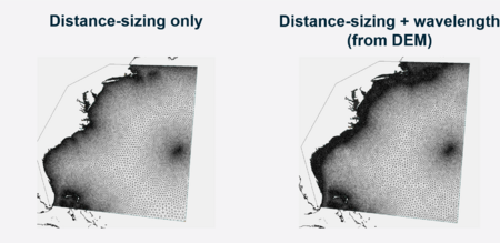 Figure 6: Comparison between a mesh generated solely using a distance-sizing function (left panel) and a mesh incorporating both distance and wavelength sizing functions (right panel). This example illustrates the element distribution according to a wavelength-to-grid scale mesh sizing function. The parameter "Number of elements per wavelength" enhances resolution on the continental shelf.
- Wavelength-to-gridscale: The local wavelength of a shallow-water wave with user-specified period is calculated (by default the period of the M2 semi-diurnal tidal constituent 12.42 hours is specified) and gravity is assumed to be 9.81 m/s^2. Elemental resolution is then determined by dividing the calculated wavelength by the “Number of elements per wavelength” parameter (by default 100). This sizing function requires a digital elevation model be specified via “Input DEM for select mesh sizing functions” option.
- Mesh sizing function #3 (optional):
- CFL Timestep Bounding: This mesh sizing function adjusts the mesh sizing function so an estimated upper bound of the Courant number is respected, assuming a user-specified simulation time step. Note this function does not act to refine the mesh in the case that a minimum Courant number is necessary, which is common in ALE schemes for example used by SCHISM. This will be incorporated in later developments.
- When to use: It is generally always encouraged to incorporate this sizing function when there is topobathymetryic data that intended to interpolate onto the mesh nodes. This encourages the numerical stability of the developed model when simulation is attempted. The Courant number is estimated through the canonical approach as the ratio of user-specified simulation time step in seconds multiplied by the shallow-water wave speed in meters per second divided by the local mesh resolution in meters. This sizing function requires a digital elevation model be specified via “Input DEM for select mesh sizing functions” option.
- Options:
- “Maximum Allowable Timestep (seconds)” - The anticipated simulation time step.
- “Maximum Allowable Courant Number for given timestep” – The upper bound Courant number that will violate the CFL condition of the numerical scheme.
- The tool constructs each sizing function independently, then computes their spatial minimum to synthesize the "final mesh sizing function."
- CFL Timestep Bounding: This mesh sizing function adjusts the mesh sizing function so an estimated upper bound of the Courant number is respected, assuming a user-specified simulation time step. Note this function does not act to refine the mesh in the case that a minimum Courant number is necessary, which is common in ALE schemes for example used by SCHISM. This will be incorporated in later developments.
- Filename of mesh sizing function – the final mesh sizing function used to generate the mesh is exported as a geotiff. Note this file will automatically visualize after execution of the tool inside SMS.
- Modify the mesh cleaning options (optional) – By default several mesh cleaning routines are enabled to ensure a higher quality mesh is developed which can be advantageous for numerical simulation.
- Options (all options can be turned off by setting them to 0):
- “Minimum boundary quality” – All boundary elements with a mesh quality () less than this threshold will be deleted.
- “Disconnected areas with this percent of the total area are removed” – Portions of the mesh that are disconnected with an area less than this percent of the total mesh will be deleted. For example, removing disconnected inland lakes when meshing a coastal domain.
- “Maximum number of iterations for Laplace smoothing” – The maximum number of iterations to apply Laplace smoothing. Move vertices to the average position of their connected neighbours.
- “Minimum movement tolerance for Laplace smoothing” – If an iteration of Laplace smoothing produces a nodal movement less than this tolerance, iterations will cease.
- Options (all options can be turned off by setting them to 0):
- “Modify mesh generation options”: Users should only modify the following force functions if their mesh is not convergent and not producing a relatively high-quality discretization. In this case, it makes sense to increase the number of iterations 25 to 50% while lowering the pseudo timestep 25 to 50% and switching the force function to “person_strang” from the default “bossen_heckbert”.
- Options:
- “Number of meshing iterations” – Number of meshing iterations to perform. Generally, more iterations imply a higher mesh quality at the cost of more time spent meshing. With that said almost all problems encountered saturate around 100 iterations.
- “Pseudo timestep for meshing” – Mesh generation is solved using a force-balance approach (Roberts et al. 2019) that time marches the solution to a system of ordinary differential equations. Depending on the stiffness of the problem, the time step can be modified to achieve better results. Generally, if meshing is not convergent, then halving the time step is recommended. If meshing is converging rapidly in say less than 25 iterations, it may be possible to double the time step and achieve better resulrts. A suitable range is between 0.05 and 0.20 pseudo seconds.
- Nodes are moved iteratively. Forces originate based on discrepancy between the edge lengths of the current triangulation and the mesh sizing function.
- “Force function used in mesh generation”.
- “persson_strang”- Nodes move according to a linear spring repulsion based on Hooke’s Law.
- “bossen_heckbert” – Nodes move according to a non-linear electrostatic attraction and repulsion function. This is the default and generally produces higher quality meshes at termination than “person_strang”.
- “persson_strang”- Nodes move according to a linear spring repulsion based on Hooke’s Law.
- “Force function used in mesh generation”.
- Options:
- Filename of generate mesh – the filename of the generated mesh. The mesh will automatically visualize after successful execution of the tool.
Outputs
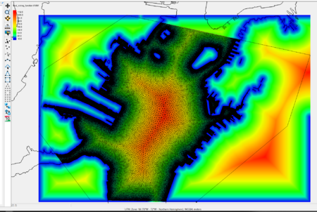
Name of the 2D triangular unstructured mesh that will be generated. A mesh will be visualized in the SMS GUI along with the sizing function as a contour filled image appearing behind the mesh.
Current Location in Toolbox
Unstructured Grids/OceanMesh UGrid from Coverage
References
- Randolph E. Bank. PLTMG: A Software Package for Solving Elliptic Partial Differential Equations. Society for Industrial and Applied Mathematics, 1 1998. ISBN 978-0-89871-409-8. doi: 10.1137/ 1.9780898719635. URL http://epubs.siam.org/doi/book/10.1137/1.9780898719635.
- Ocean Mesh 2D on Github
- Roberts, K. J., Pringle, W. J., and Westerink, J. J., 2019. OceanMesh2D 1.0: MATLAB-based software for two-dimensional unstructured mesh generation in coastal ocean modeling, Geosci. Model Dev. (GMD), https://doi.org/10.5194/gmd-12-1847-2019.
- Persson, Per-Olof. "PDE-Based Gradient Limiting for Mesh Size Functions." IMR. 2004.
