User:Jcreer/MDOFLOW 6 New Packages: Difference between revisions
| Line 491: | Line 491: | ||
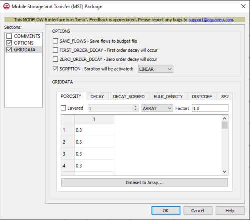
** ''FIRST_ORDER_DECAY'' – This indicates that first-order decay will occur. This requires that ''DECAY'' and ''DECAY_SORBED'' (if ''SORPTION'' has been specified) are specified in the ''GRIDDATA'' section. | ** ''FIRST_ORDER_DECAY'' – This indicates that first-order decay will occur. This requires that ''DECAY'' and ''DECAY_SORBED'' (if ''SORPTION'' has been specified) are specified in the ''GRIDDATA'' section. | ||
** ''ZERO_ORDER_DECAY'' – This indicates that zero-order decay will occur. This requires that ''DECAY'' and ''DECAY_SORBED'' (if ''SORPTION'' has been specified) are specified in the ''GRIDDATA'' section. | ** ''ZERO_ORDER_DECAY'' – This indicates that zero-order decay will occur. This requires that ''DECAY'' and ''DECAY_SORBED'' (if ''SORPTION'' has been specified) are specified in the ''GRIDDATA'' section. | ||
** ''SORPTION'' – | ** ''SORPTION'' – This indicates that sorption will be activated. This requires that ''BULK_DENSITY'' and ''DISTCOEF'' are specified in the ''GRIDDATA'' section. This will also activate a drop-down where the type of sorption can be chosen, from the following options: | ||
*** "LINEAR" | *** "LINEAR" | ||
*** "FREUNDLICH" | *** "FREUNDLICH" | ||
*** "LANGMUIR" | *** "LANGMUIR" | ||
*''GRIDDATA'' section – This deals with the ''GRIDDATA'' block. | *''GRIDDATA'' section – This deals with the ''GRIDDATA'' block. | ||
** ''Define'' – This allows data within the ''GRIDDATA'' section to be defined. When this is inactive, all of the options within a given tab are grayed out. This option is specifically available in all of the tabs except for the ''POROSITY'' tab. In the ''POROSITY'' tab, it is not visible but automatically activated so all the options are activated. | |||
** ''Define'' – This allows data within the ''GRIDDATA'' section to be defined. When this is inactive, all of the options within a given tab are grayed out. This option is | |||
** '''Dataset to Array...''' – This button brings up a ''Select Dataset'' dialog, where a single dataset can be selected for use in the ''GRIDDATA'' section. This will populate its spreadsheet. This option is grayed out if ''Define'' is not turned on. | ** '''Dataset to Array...''' – This button brings up a ''Select Dataset'' dialog, where a single dataset can be selected for use in the ''GRIDDATA'' section. This will populate its spreadsheet. This option is grayed out if ''Define'' is not turned on. | ||
** ''Layered'' – When this is active, a numeric updown for the layers will become available. | ** ''Layered'' – When this is active, a numeric updown for the layers will become available. | ||
| Line 503: | Line 502: | ||
*** "CONSTANT" – This will change the textbox to the right to be representative of "Constant". If this is selected, the spreadsheet in the ''GRIDDATA'' section will be grayed out. | *** "CONSTANT" – This will change the textbox to the right to be representative of "Constant". If this is selected, the spreadsheet in the ''GRIDDATA'' section will be grayed out. | ||
*** "ARRAY" – This will change the textbox to the right to be representative of "Factor". If this is selected, the spreadsheet in the ''GRIDDATA'' section will not be grayed out, and its cells will be editable. | *** "ARRAY" – This will change the textbox to the right to be representative of "Factor". If this is selected, the spreadsheet in the ''GRIDDATA'' section will not be grayed out, and its cells will be editable. | ||
** ''POROSITY'' – | ** ''POROSITY'' – The ''POROSITY'' tab represents the aquifer porosities. | ||
** ''DECAY'' – | ** ''DECAY'' – The ''DECAY'' tab represents the rate coefficients for first/zero-order decay for the aqueous phase of the mobile domain. Negative values indicate solute production. For first-order decay, the dimensions of ''DECAY'' is one over time. For zero-order decay, the dimensions of ''DECAY'' is mass per length cubed per time. If neither ''FIRST_ORDER_DECAY'' nor ''ZERO_ORDER_DECAY'' are specified, then ''DECAY'' will have no impact on simulation results. | ||
** ''DECAY_SORBED'' – | ** ''DECAY_SORBED'' – The ''DECAY_SORBED'' tab represents the rate coefficients for first/zero-order decay for the sorbed phase of the mobile domain. Negative values indicate solute production. For first-order decay, the dimension of ''DECAY_SORBED'' is one over time. For zero-order decay, the dimensions of ''DECAY_SORBED'' is mass of solute per mass of aquifer per time. If ''DECAY_SORBED'' is not specified, but both ''DECAY'' and ''SORPTION'' are active, the sorbed decay rate will be set to the same value as the aqueous decay rate. If ''SORPTION'' hasn't been specified and neither ''FIRST_ORDER_DECAY'' nor ''ZERO_ORDER_DECAY'' have been specified, then ''DECAY_SORBED'' will have no impact on simulation results. | ||
** ''BULK_DENSITY'' – | ** ''BULK_DENSITY'' – The ''BULK_DENSITY'' tab represents the bulk densities of the aquifer in mass per length cubed. If ''SORPTION'' hasn't been specified, then BULK_DENSITY will not be required. | ||
** ''DISTCOEF'' – | ** ''DISTCOEF'' – The ''DISTCOEF'' tab represents the distribution coefficients for the equilibrium-controlled linear sorption isotherm in dimensions of length cubed per mass. If ''SORPTION'' hasn't been specified, then ''DISTCOEF'' will not be required. | ||
** ''SP2'' – | ** ''SP2'' – ??? | ||
{{-}} | {{-}} | ||
Revision as of 18:50, 23 July 2021
| This contains information about functionality available starting at GMS version 10.6. The content may not apply to other versions. |
MF6 BUY Package
The Buoyancy (BUY) Package dialog is accessed by double-clicking on the BUY package under a MODFLOW 6 simulation in the Project Explorer. It contains the following sections and options:
- Sections list – A list of sections that can be turned on or off:
- COMMENTS – Turn on to make the COMMENTS section visible.
- OPTIONS – Turn on to make the OPTIONS section visible.
- PACKAGEDATA – Turn on to make the PACAKGEDATA section visible. This section is on by default.
- COMMENTS section – Enter general alphanumeric comments. Comments entered here get written at the top of the file, preceded by a '#' symbol.
- OPTIONS section – Temporal options and settings:
- HHFORMULATION_RHS – Using variable-density hydraulic head formulation on the right-hand, this prevents adding asymmetric terms to the flow matrix.
- DENSEREF – This allows a fluid reference density to be specified in the equation of state. If not active to be specified, this value is set to 1000.
- DENSITY FILEOUT – This allows the density to be saved to a binary output file that is specified.
- PACKAGEDATA section – This deals with the PACKAGEDATA block. It is a spreadsheet section which contains the following:
- Add Rows... – This button brings up a Rows to Add dialog, where a number can be specified in the numeric updown to the right of Number of rows to add at bottom. This will help populate the spreadsheet.
- IRHOSPEC – This column represents the IRHOSPEC integer values, which define the species numbers for the PACKAGEDATA on each line. These must be greater than zero and less than or equal to the separately defined NRHOSPECIES value. The program will terminate with an error if an NRHOSPECIES species doesn't have information specified, or if its information is specified more than once.
- DRHODC – This column represents the DRHODC values, which define the slopes of the density-concentration lines used in the density equation of state.
- CRHOREF – This column represents the CRHOREF values, which define the reference concentration values used in the density equation of state.
- MODELNAME – This column represents the MODELNAME values, which names the GWT models that will be used to simulate species in the density equation of state. This will only work if the simulation includes a GWT model that corresponds to the name.
- AUXSPECIESNAME – This column represents the AUXSPECIESNAME values, which names GWF stress package auxiliary variables that will be used to calculate a density value. The Buoyancy Package can use these simulated concentration values to calculate density values for lakes, streams, multi-aquifer wells, and unsaturated zone flow cells.
MF6 CSUB Package
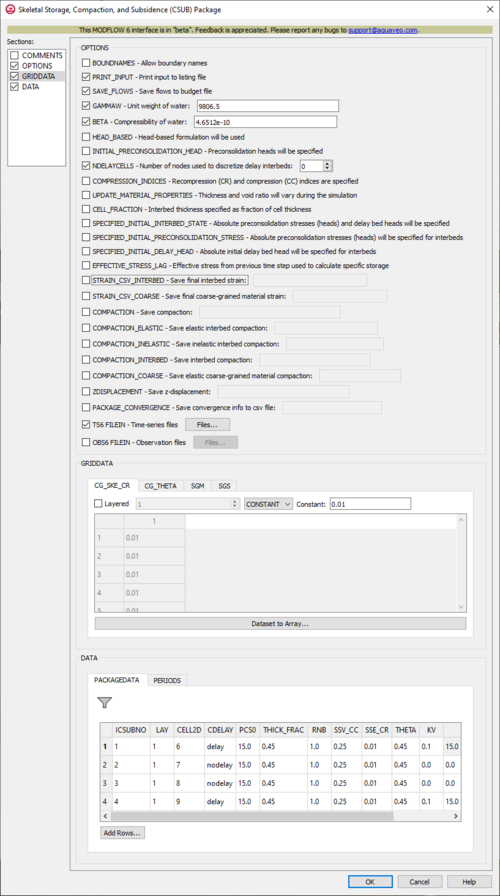
The Skeletal Storage, Compaction, and Subsidence (CSUB) Package dialog is accessed by double-clicking on the CSUB package under a MODFLOW 6 simulation in the Project Explorer. It contains the following sections and options:
- Sections list – A list of sections that can be turned on or off:
- COMMENTS – Turn on to make the COMMENTS section visible.
- OPTIONS – Turn on to make the OPTIONS section visible.
- GRIDDATA – Turn on to make the GRIDDATA section visible.
- DATA – Turn on to make the DATA section visible. This section is on by default.
- COMMENTS section – Enter general alphanumeric comments. Comments entered here get written at the top of the file, preceded by a '#' symbol.
- OPTIONS section – Options and settings:
- BOUNDNAMES – This allows for boundary names to be provided with the list of CSUB cells.
- PRINT_INPUT – This indicates that the list of CSUB input will be printed to the listing file immediately after it is read.
- SAVE_FLOWS – This indicates that cell-by-cell flow terms will be saved to a budget file (specified in Output Control with "BUDGET SAVE FILE").
- GAMMAW – This allows the unit weight of water to be set. For freshwater, GAMMAW is 9806.65 Newtons/cubic meters (SI) or 62.48 lb/cubic foot (English units). The default value for GAMMAW is 9806.65 Newtons/cubic meters.
- BETA – This allows for the compressibility of water to be set. Typical values of BETA are 4.6512e-10 1/Pa (SI) or 2.2270e-8 lb/square foot (English units). The default value for BETA is 4.6512e-10 1/Pa.
- HEAD_BASED – This indicates that head-based formulation will be used to simulate coarse-grained aquifer materials and no-delay and delay interbeds. If specified, then INITIAL_PRECONSOLIDATION_HEAD will be as well.
- INITIAL_PRECONSOLIDATION_HEAD – This indicates that preconsolidation heads will be specified for no-delay and delay interbeds in the PACKAGEDATA block. When SPECIFIED_INTIAL_INTERBED_STATE is specified, these will be absolute values. When it isn't, these will be relative to steady-state or initial heads.
- NDELAYCELLS – This allows a number to be set for the number of nodes used to discretize delay interbeds. When this isn't set, a default value of 19 is assigned.
- COMPRESSION_INDICES – This indicates that recompression (CR) and compression (CC) indices will be specified, replacing the elastic specific storage (SSE) and inelastic specific storage (SSV) coefficients. When this isn't set, the SSE and SSV coefficients will have to be specified.
- UPDATE_MATERIAL_PROPERTIES – This indicates that the thickness and void ratio of coarse-grained and interbed sediments (delay and no-delay) will vary during the simulation. When this isn't set, the ratio will not vary during the simulation.
- CELL_FRACTION – This indicates that interbed thickness will be specified as a fraction of cell thickness. When this isn't set, the interbed thickness will have to be individually specified.
- SPECIFIED_INITIAL_INTERBED_STATE – This indicates that absolute preconsolidation stresses (heads) and delay bed heads will be specified for the interbeds that are defined in the PACKAGEDATA block. This is equivalent to specifying both SPECIFIED_INITIAL_PRECONSOLDIATION_STRESS and SPECIFIED_INITIAL_DELAY_HEAD. If this option is not set, then these values will be relative to simulated values (if the first stress period is steady-state) or initial stresses and GWF heads (if the first stress period is transient).
- SPECIFIED_INITIAL_PRECONSOLIDATION_STRESS – This indicates that absolute preconsolidation stresses (heads) will be specified for interbeds that are defined in the PACKAGEDATA block. If neither this option nor SPECIFIED_INITIAL_INTERBED_STATE are set, then these values will be relative to simulated values (if the first stress period is steady-state) or initial stresses (heads) (if the first stress period is transient).
- SPECIFIED_INITIAL_DELAY_HEAD – This indicates that absolute initial delay bed head will be specified for interbeds that are defined in the PACKAGEDATA block. If neither this option nor SPECIFIED_INITIAL_INTERBED_STATE are set, then these values will be relative to simulated values (if the first stress period is steady-state) or initial GWF heads (if the first stress period is transient).
- EFFECTIVE_STRESS_LAG – This indicates that effective stress from the previous time step will be used to calculate specific storage values. This is helpful with convergence in models with thin cells and water table elevations close to land surface, is identical to the SUBWT package approach for MODFLOW-2005, and will only be used when the effective-stress formulation is being used. When this isn't set, the default is to use current effective stress values to calculate specific storage values.
- STRAIN_CSV_INTERBED – This allows the final interbed strain output to be saved to a specified file.
- STRAIN_CSV_COARSE – This allows the final coarse-grained material strain output to be saved to a specified file.
- COMPACTION – This allows the compaction to be saved to a specified file.
- COMPACTION_ELASTIC – This allows the elastic interbed compaction to be saved to a specified binary file.
- COMPACTION_INELASTIC – This allows the inelastic interbed compaction to be saved to a specified binary file.
- COMPACTION_INTERBED – This allows the interbed compaction to be saved to a specified binary file.
- COMPACTION_COARSE – This allows the elastic coarse-grained material compaction to be saved to a specified binary file.
- ZDISPLACEMENT – This allows the z-displacement to be saved to a specified binary file.
- PACKAGE_CONVERGENCE – This allows the package convergence info to be saved to a comma-separated values (CSV) file.
- TS6 FILEIN – This allows time series files to be used as input to assign time-varying values. Specifying this option will allow a Files... button to its right to be clicked. Doing so will bring up a Files dialog. In this dialog, a spreadsheet can be filled in that has two columns. The following options can be used to help develop the spreadsheet:
- Insert Row – This will insert a new row at the current location.
- Add Row – This will add a new row at the bottom.
- Delete Row – This will delete the currently selected row.
- Move Up – This will move the currently selected row up a row.
- Move Down – This will move the currently selected row down a row.
- OBS6 FILEIN – This allows observations files to be used as input. Specifying this option will allow a Files... button to its right to be clicked. Doing so will bring up a Files dialog. In this dialog, a spreadsheet can be filled in that has two columns. The first column allows filenames to be specified. The second column has an Edit... button relating to the file specified. The following options can be used to help develop the spreadsheet:
- Insert Row – This will insert a new row at the current location.
- Add Row – This will add a new row at the bottom.
- Delete Row – This will delete the currently selected row.
- Move Up – This will move the currently selected row up a row.
- Move Down – This will move the currently selected row down a row.
- GRIDDATA section – This deals with the GRIDDATA block.
- Dataset to Array... – This button brings up a Select Dataset dialog, where a single dataset can be selected for use in the GRIDDATA section. This will populate its spreadsheet. This option is grayed out if Define is not turned on. The CG_SKE_CR and CG_THETA tabs do not have the Define option visible, so the button is always available for them.
- Define – This allows data within the GRIDDATA section to be defined. When this is inactive, all of the options within a given tab are grayed out. This option is unavailable in the CG_SKE_CR and CG_THETA tabs, so they are automatically defined.
- Layered – When this is active, a numeric updown for the layers will become available.
- Drop-down and Constant/Factor – The drop-down in the GRIDDATA section has two options. The option selected will change the nature of the textbox to its right.
- "CONSTANT" – This will change the textbox to the right to be representative of "Constant". If this is selected, the spreadsheet in the GRIDDATA section will be grayed out.
- "ARRAY" – This will change the textbox to the right to be representative of "Factor". If this is selected, the spreadsheet in the GRIDDATA section will not be grayed out, and its cells will be editable.
- CG_SKE_CR – The CG_SKE_CR tab represents either the initial elastic coarse-grained material specific storage of recompression index. If COMPRESSION_INDICES was set, then this will represent the recompression index. Otherwise this will represent the elastic specific storage. If HEAD_BASED was set, then specified/calculated elastic coarse-grained material specific storage values will not be adjusted from the initial values.
- CG_THETA – The CG_THETA tab represents the initial porosity of coarse-grained materials.
- SGM – The SGM tab represents the specific gravity of moist or unsaturated sediments. When this isn't specified, a default value of 1.7 will be used.
- SGS – The SGS tab represents the specific gravity of saturated sediments. When this isn't specified, a default value of 2.0 will be used.
- DATA section – Contains the following tabs:
- PACKAGEDATA – This deals with the PACKAGEDATA block.
- Add Rows... – This button brings up a Rows to Add dialog, where a number can be specified to the right of Number of rows to add at bottom. This will help populate the spreadsheet.
- Filter on Selected Cells – ???
- ICSUBNO – This column represents the ICSUBNO integer values, which define the CSUB interbed numbers for the PACKAGEDATA on each line. The CSUBNO values must be greater than zero and less than or equal to the separately defined NINTERBEDS value. The program will terminate with an error if a CSUB cell doesn't have information specified, or if information for a CSUB interbed number is specified more than once.
- CELLID – This will display differently in the spreadsheet based on what type of grid is used for the simulation, specifically which type of DIS* input file is used in the model. The CELLID is the cell identifier, and the type of DIS* file used will change what will be determined to be the CELLID.
- For a structured grid that uses a DIS input file, these columns will be:
- LAY – This column represents the layers of the cells.
- ROW – This column represents the rows of the cells.
- COL – This column represents the columns of the cells.
- For a grid that uses a DISV input file, these columns will be:
- LAY – This column represents the layers of the cells.
- CELL2D – This column represents the CELL2D numbers of the cells.
- If the model uses a DISU (unstructured discretization) file, the column will be:
- CELLID – This column represents the node numbers of the cells.
- For a structured grid that uses a DIS input file, these columns will be:
- CDELAY – This column represents the CDELAY character strings, which define the subsidence package delay type for the interbeds. Possible CDELAY strings include:
- "NODELAY" – Character keyword that indicates delay will not be simulated in the interbed.
- "DELAY" – Character keyword that indicates delay will be simulated in the interbed.
- PCS0 – This column represents the PCS0 values, which are the initial offsets from the calculated initial effective/preconsolidation stress in the interbeds, in the units of the height of a column of water. If SPECIFIED_INITIAL_INTERBED_STATE or SPECIFIED_INITIAL_PRECONSOLIDATION_STRESS have been specified, then these are the initial preconsolidation stresses. If HEAD_BASED is set, then these are the initial offsets from the calculated initial head/preconsolidation heads in the CSUB interbeds, and initial preconsolidation stresses are calculated from the calculated initial effective/geostatic stresses.
- THICK_FRAC – This column represents the THICK_FRAC values, which are the interbed thickness/cell fractions of the interbeds. If CELL_FRACTION has been specified, interbed thickness is specified as a fraction of the cell thickness.
- RNB – This column represents the RNB values, which are the interbed material factor equivalent numbers of interbeds in the interbed systems represented by the interbeds. If CDELAY has been set to "DELAY", these values must be greater than or equal to 1. If not, then these values can be any value.
- SSV_CC – This column represents the SSV_CC values, which are the initial inelastic specific storages or compression indexes of the interbeds. If COMPRESSION_INDICES is set, then the compression index is specified. If HEAD_BASED is set, then specified/calculated interbed inelastic specific storage values are not adjusted from the initial values.
- SSE_CR – This column represents the SSE_CR values, which are the initial elastic coarse-grained material specific storages or recompression indexes of the interbeds. If COMPRESSION_INDICES is set, then the recompression index is specified. If HEAD_BASED is set, then the specified/calculated interbed elastic specific storage values are not adjusted from the initial values.
- THETA – This column represents the THETA values, which are the initial porosities of the interbeds.
- KV – This column represents the KV values, which are the vertical hydraulic conductivities of the delay interbeds. If CDELAY has been set to "DELAY", these must be greater than 0. If not, then these values can be any value.
- H0 – This column represents the H0 values, which are the initial offsets from the heads in cell CELLIDs or the initial heads in the delay interbeds. If SPECIFIED_INITIAL_INTERBED_STATE or SPECIFIED_INITIAL_DELAY_HEAD are set, then these are the initial heads in the delay beds. If CDELAY has been set to "NODELAY", then these can be any value.
- PERIODS – This deals with the PERIODS block.
- Period – A numeric updown can be used to enter which period is being examined in the spreadsheet.
- Define Period – This button will allow a period to be defined. This will be active when no period has yet been defined, and it may gray out once one has been created.
- Delete Period – This button will delete the selected period. A dialog warning will come up first asking the user to confirm their decision to delete the period.
- Add Rows – This button will bring up an Add Stresses dialog. The following options can be used to help in adding the stresses:
- Columns and Values – Numeric updowns and textboxes can be used to enter the values for their relevant columns for all the new stresses. These may include columns that are not actually present in the spreadsheet.
- Number of rows to add – A numeric updown can be used to enter the number of rows that will be added to the spreadsheet.
- Add to – There are two different options, only one of which can be selected at a time.
- All defined periods – These stresses will be added to all the periods that have been defined.
- Only this period – These stresses will be added only to the currently selected period.
- Delete Rows – This button will delete all of the stresses. A dialog warning will come up first asking the user to confirm their decision to delete the stresses. The dialog will also give them the option to either Delete From All Periods or Delete From Just This Period.
- Plot All Periods – This will allow the user to plot all the periods that have been defined.
- Open Time Series – This will allow the user to open a time series file.
- The columns listed in the spreadsheet will differ, based on which type of DIS* input file is used in the model.
- If the model uses a DIS input file, these columns will be:
- LAY – This column represents the layers of the cells.
- ROW – This column represents the rows of the cells.
- COL – This column represents the columns of the cells.
- SIG0 – This column represents the stress offsets for the cells. SIG0 is added to the calculated geostatic stresses for the cells. SIG0 will only be specified if a separately defined MAXSIG0 value is set to be greater than 0. If time series files are used as input, entering a time series name instead of a numeric value can allow for values to be obtained from a time series.
- If the model uses a DISV input file, these columns will be:
- LAY – This column represents the layers of the cells.
- ROW – This column represents the rows of the cells.
- COL – This column represents the columns of the cells.
- If the model uses a DISU input file, these columns will be:
- LAY – This column represents the layers of the cells.
- ROW – This column represents the rows of the cells.
- If the model uses a DIS input file, these columns will be:
- PACKAGEDATA – This deals with the PACKAGEDATA block.
MF6 ADV Package
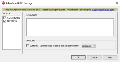
The Advection (ADV) Package dialog is accessed by double-clicking on the ADV package under a MODFLOW 6 simulation in the Project Explorer. It contains the following sections and options:
- Sections list – A list of sections that can be turned on or off:
- COMMENTS – Turn on to make the COMMENTS section visible.
- OPTIONS – Turn on to make the OPTIONS section visible.
- COMMENTS section – Enter general alphanumeric comments. Comments entered here get written at the top of the file, preceded by a '#' symbol.
- OPTIONS section – Options and settings:
- SCHEME – This drop-down can be used to select which weighting scheme will be used to solve the advection term. There are three options:
- "upstream" – An upstream weighting scheme will be used. This is the default option.
- "central" – A central weighting scheme will be used.
- "TVD" – A TVD weighting scheme will be used.
- SCHEME – This drop-down can be used to select which weighting scheme will be used to solve the advection term. There are three options:
MF6 CNC Package
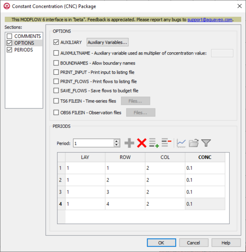
The Constant Concentration (CNC) Package dialog is accessed by double-clicking on the CNC package under a MODFLOW 6 simulation in the Project Explorer. It contains the following sections and options:
- Sections list – A list of sections that can be turned on or off:
- COMMENTS – Turn on to make the COMMENTS section visible.
- OPTIONS – Turn on to make the OPTIONS section visible.
- PERIODS – Turn on to make the PERIODS section visible.
- COMMENTS section – Enter general alphanumeric comments. Comments entered here get written at the top of the file, preceded by a '#' symbol.
- OPTIONS section – Options and settings:
- AUXILIARY – This allows an array of one or more auxiliary variables to be named. There are no limits to the number of auxiliary variables that can be provided, but subsequent blocks will require data for each of the auxiliary variables that are defined. Turning this on will activate an Auxiliary Variables... button. Clicking the button will bring up an Auxiliary Variables dialog. The following options can be used to help develop the auxiliary variables:
- Insert Row – This will insert a new row at the current location.
- Add Row – This will add a new row at the bottom.
- Delete Row – This will delete the currently selected row.
- Move Up – This will move the currently selected row up a row.
- Move Down – This will move the currently selected row down a row.
- AUXMULTNAME – This allows for an auxiliary variable to be used as a multiplier of concentration value. A textbox to the right of the option can be used to specify the name.
- BOUNDNAMES – This indicates that boundary names are allowed to be provided with the list of constant concentration cells. This will add the BOUNDNAME column to the spreadsheet in the PERIODS section.
- PRINT_INPUT – This indicates that the list of constant concentration information input will be printed to the listing file immediately after it is read.
- PRINT_FLOWS – This indicates that the list of constant concentration flow rates will be printed to the listing file. Flow rates will be printed for the last time step of each stress period.
- SAVE_FLOWS – This indicates that constant concentration flow terms will be saved to a budget file (specified in Output Control with "BUDGET FILEOUT").
- TS6 FILEIN – This allows time series files to be used as input to assign time-varying values. Specifying this option will allow a Files... button to its right to be clicked. Doing so will bring up a Files... dialog. In this dialog, a spreadsheet can be filled in that has two columns. The following options can be used to help develop the spreadsheet:
- Insert Row – This will insert a new row at the current location.
- Add Row – This will add a new row at the bottom.
- Delete Row – This will delete the currently selected row.
- Move Up – This will move the currently selected row up a row.
- Move Down – This will move the currently selected row down a row.
- OBS6 FILEIN – This allows observations files to be used as input. Specifying this option will allow a Files... button to its right to be clicked. Doing so will bring up an Observation Files dialog. In this dialog, a spreadsheet can be filled in that has two columns. The first column allows filenames to be specified. The second column has an Edit... button relating to the file specified. The following options can be used to help develop the spreadsheet:
- Insert Row – This will insert a new row at the current location.
- Add Row – This will add a new row at the bottom.
- Delete Row – This will delete the currently selected row.
- Move Up – This will move the currently selected row up a row.
- Move Down – This will move the currently selected row down a row.
- AUXILIARY – This allows an array of one or more auxiliary variables to be named. There are no limits to the number of auxiliary variables that can be provided, but subsequent blocks will require data for each of the auxiliary variables that are defined. Turning this on will activate an Auxiliary Variables... button. Clicking the button will bring up an Auxiliary Variables dialog. The following options can be used to help develop the auxiliary variables:
- PERIODS section – This deals with the PERIODS block.
- Period – A numeric updown can be used to enter which period is being examined in the spreadsheet.
- Define Period – This button will allow a period to be defined. This will be active when no period has yet been defined, and it may gray out once one has been created.
- Delete Period – This button will delete the selected period. A dialog warning will come up first asking the user to confirm their decision to delete the period.
- Add Rows – This button will bring up an Add Stresses dialog. The following options can be used to help in adding the stresses:
- Columns and Values – Numeric updowns and textboxes can be used to enter the values for their relevant columns for all the new stresses. These may include columns that are not actually present in the spreadsheet.
- Number of rows to add – A numeric updown can be used to enter the number of rows that will be added to the spreadsheet.
- Add to – There are two different options, only one of which can be selected at a time.
- All defined periods – These stresses will be added to all the periods that have been defined.
- Only this period – These stresses will be added only to the currently selected period.
- Delete Rows – This button will delete all of the stresses. A dialog warning will come up first asking the user to confirm their decision to delete the stresses. The dialog will also give them the option to either Delete From All Periods or Delete From Just This Period.
- Plot All Periods – This will allow the user to plot all the periods that have been defined.
- Open Time Series – This will allow the user to open a time series file.
- Filter on Selected Cells – ???
- CELLID – This will display differently in the spreadsheet based on what type of grid is used for the simulation, specifically which type of DIS* input file is used in the model. The CELLID is the cell identifier, and the type of DIS* file used will change what will be determined to be the CELLID.
- For a structured grid that uses a DIS input file, these columns will be:
- LAY – This column represents the layers of the cells.
- ROW – This column represents the rows of the cells.
- COL – This column represents the columns of the cells.
- For a grid that uses a DISV input file, these columns will be:
- LAY – This column represents the layers of the cells.
- CELL2D – This column represents the CELL2D numbers of the cells.
- If the model uses a DISU (unstructured discretization) file, the column will be:
- CELLID – This column represents the node numbers of the cells.
- For a structured grid that uses a DIS input file, these columns will be:
- CONC – This column represents the constant concentration values. If time series files are used as input, entering a time series name instead of a numeric value can allow for values to be obtained from a time series.
- AUX – These columns represent the values of the auxiliary variables for each constant concentration, which previously may have been created if the AUXILIARY option was set. If time series files are used as input, entering a time series name instead of a numeric value can allow for values to be obtained from a time series.
- BOUNDNAME – This column represents the names of the constant concentration cells, and will appear if the BOUNDNAMES option was set. BOUNDNAME values are ASCII character variables that can contain as many as 40 characters. If a BOUNDNAME value contains spaces within it, then the entire name will have to be enclosed within single quotes.
MF6 DSP Package
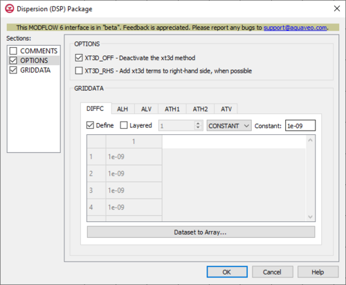
The Dispersion (DSP) Package dialog is accessed by double-clicking on the DSP package under a MODFLOW 6 simulation in the Project Explorer. It contains the following sections and options:
- Sections list – A list of sections that can be turned on or off:
- COMMENTS – Turn on to make the COMMENTS section visible.
- OPTIONS – Turn on to make the OPTIONS section visible.
- GRIDDATA – Turn on to make the GRIDDATA section visible.
- COMMENTS section – Enter general alphanumeric comments. Comments entered here get written at the top of the file, preceded by a '#' symbol.
- OPTIONS section – Options and settings:
- XT3D_OFF – This deactives the XT3D method, to use the faster but less accurate approximation method. In some circumstances, the solution this provides may be fast and accurate. These could include when flow aligns with the model grid, when there is no mechanical dispersion, or when the longitudinal and transverse dispersivities are equal. This may also be useful in assessing the computational demand of the XT3D approach, by comparing run time differences with this option turned on or off.
- XT3D_RHS – This adds XT3D terms to the right-hand side, when possible. This uses less memory, but might require more iterations.
- GRIDDATA section – This deals with the GRIDDATA block.
- Define – This allows data within the GRIDDATA section to be defined. When this is inactive in a tab, all of the options within that given tab are grayed out.
- Layered – When this is active, a numeric updown for the layers will become available.
- Drop-down and Constant/Factor – The drop-down in the GRIDDATA section has two options. The option selected will change the nature of the textbox to its right.
- "CONSTANT" – This will change the textbox to the right to be representative of "Constant". If this is selected, the spreadsheet in the GRIDDATA section will be grayed out.
- "ARRAY" – This will change the textbox to the right to be representative of "Factor". If this is selected, the spreadsheet in the GRIDDATA section will not be grayed out, and its cells will be editable.
- Dataset to Array... – This button brings up a Select Dataset dialog, where a single dataset can be selected for use in the GRIDDATA section. This will populate its spreadsheet. This option is grayed out if Define is not turned on.
- DIFFC – The DIFFC tab represents the effective molecular diffusion coefficients.
- ALH – The ALH tab represents the longitudinal dispersivities in the horizontal direction. When flow is strictly horizontal, these are the longitudinal dispersivities that will be used. When flow is neither strictly horizontal nor vertical, then the longitudinal dispersivity will be a function of both ALH and ALV. An ALH array is required when mechanical dispersion is represented (by specifying any dispersivity values).
- ALV – The ALV tab represents the longitudinal dispersivities in the vertical direction. When flow is strictly vertical, these are the longitudinal dispersivities that will be used. When flow is neither strictly horizontal nor vertical, then the longitudinal dispersivity will be a function of both ALH and ALV. An ALV array will be set set equal to an ALH array when its value is not specified and mechanical dispersion is represented.
- ATH1 – The ATH1 tab represents the transverse dispersivities in the horizontal direction. These are the transverse dispersivity values for the second ellipsoid axis. When flow is strictly horizontal and directed in the X direction (along a row for a regular grid), then these values control spreading in the Y direction. An ATH1 array is required when mechanical dispersion is represented (by specifying any dispersivity values).
- ATH2 – The ATH2 tab represents the transverse dispersivities in the horizontal direction. These are the transverse dispersivity values for the third ellipsoid axis. When flow is strictly horizontal and directed in the X direction (along a row for a regular grid), then these values control spreading in the Z direction. An ATH2 array will be set equal to an ATH1 array when its value is not specified and mechanical dispersion is represented.
- ATV – The ATV tab represents the transverse dispersivities when the flow is in the vertical direction. When flow is strictly vertical and directed in the Z direction, then these values control spreading in the X and Y directions. An ATV array will be set equal to an ATH2 array when its value is not specified and mechanical dispersion is represented.
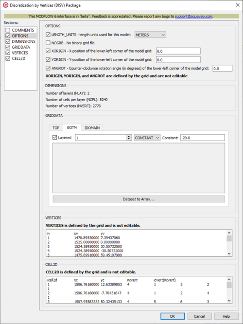
MF6 DISV Package
The Discretization by Vertices (DISV) Package dialog is accessed by double-clicking on the DISV package under a MODFLOW 6 simulation in the Project Explorer. It contains the following sections and options:
- Sections list – A list of sections that can be turned on or off:
- COMMENTS – Turn on to make the COMMENTS section visible.
- OPTIONS – Turn on to make the OPTIONS section visible.
- DIMENSIONS – Turn on to make the DIMENSIONS section visible.
- GRIDDATA – Turn on to make the GRIDDATA section visible.
- VERTICES – Turn on to make the VERTICES section visible.
- CELL2D – Turn on to make the CELL2D section visible.
- COMMENTS section – Enter general alphanumeric comments. Comments entered here get written at the top of the file, preceded by a '#' symbol.
- OPTIONS section – Options and settings:
- LENGTH_UNITS – This allows for the length units for the model to be specified. Turning it on will activate a drop-down, with the following options:
- "FEET"
- "METERS"
- "CENTIMETERS"
- "UNKNOWN" – The default value if no other one is specified.
- NOGRB – This indicates to deactivate writing of the binary grid file, so there will not be one.
- XORIGIN – This indicates the X-position of the origin used for the model grid vertices (this value is defined by the grid and is not editable). Turning it on will activate a textbox where its value (for the X-position of the lower-left corner of the model grid) will be displayed. This value should be provided in a real-world coordinate system. This value does not affect the model simulation, but is written to the binary grid file so that postprocessors will be able to locate the grid in space. If this value hasn't been set, a default value of 0.0 will be used.
- YORIGIN – This indicates the Y-position of the origin used for the model grid vertices (this value is defined by the grid and is not editable). Turning it on will activate a textbox where its value (for the Y-position of the lower-left corner of the model grid) will be displayed. This value should be provided in a real-world coordinate system. This value does not affect the model simulation, but is written to the binary grid file so that postprocessors will be able to locate the grid in space. If this value hasn't been set, a default value of 0.0 will be used.
- ANGROT – This indicates the counter-clockwise rotation angle (in degrees) of the model grid coordinate system relative to a real-world coordinate system (this value is defined by the grid and is not editable). Turning it on will activate a textbox where its value (for the counter-clockwise rotation angle (in degrees) of the lower-left corner of the model grid) will be displayed. This value does not affect the model simulation, but is written to the binary grid file so that postprocessors will be able to locate the grid in space. If this value hasn't been set, a default value of 0.0 will be used.
- LENGTH_UNITS – This allows for the length units for the model to be specified. Turning it on will activate a drop-down, with the following options:
- DIMENSIONS section – This deals with the DIMENSIONS block.
- Number of layers (NLAY) – This displays the number of layers in the model grid.
- Number of cells per layer (NCPL) – This displays the number of cells per layer. This is a constant value for the grid and it applies to all layers.
- Number of vertices (NVERT) – This displays the total number of (X, Y) vertex pairs used to characterize the horizontal configuration of the model grid.
- GRIDDATA section – This deals with the GRIDDATA block.
- Define – This allows data within the GRIDDATA section to be defined. When this is inactive, all of the options within a given tab are grayed out. This option is only specifically available in the IDOMAIN tab. In the BOTM tab, it is not visible but automatically activated so all the options are activated. In the TOP tab, it is not visible but automatically activated, but there are less options to work with.
- Dataset to Array... – This button brings up a Select Dataset dialog, where a single dataset can be selected for use in the GRIDDATA section. This will populate its spreadsheet. This option is grayed out if Define is not turned on. This only appears in the IDOMAIN and BOTM tabs.
- Layered – When this is active, a numeric updown for the layers will become available. This only appears in the IDOMAIN and BOTM tabs.
- Drop-down and Constant/Factor – The drop-down in the GRIDDATA section has two options. The option selected will change the nature of the textbox to its right.
- "CONSTANT" – This will change the textbox to the right to be representative of "Constant". If this is selected, the spreadsheet in the GRIDDATA section will be grayed out.
- "ARRAY" – This will change the textbox to the right to be representative of "Factor". If this is selected, the spreadsheet in the GRIDDATA section will not be grayed out, and its cells will be editable.
- TOP – The TOP tab represents the top elevations for each cell in the top model layer.
- BOTM – The BOTM tab represents the bottom elevations for each cell.
- IDOMAIN – The IDOMAIN tab represents the existence status of cells. This is optional to deal with. If it isn't specified, then all model cells exist within the solution. If the value for a cell is 0, the cell does not exist in the simulation. Input and output values will still be read and written for it, but internal to the program, it is excluded from the solution. If the value for a cell is 1, the cell exists in the simulation. If the value for a cell is -1, the cell does not exist in the simulation, however in this case the first existing cell above it will be connected to the first existing cell below it. This type of cell is referred to as a “vertical pass through” cell.
- VERTICES section – This deals with the VERTICES block. This section is defined by the grid and is not editable.
- iv – This column represents the iv values, which are the vertex numbers. The records in this block must be listed in consecutive order from 1 to the value defined by Number of vertices (NVERT) in the DIMENSIONS section.
- xv – This column represents the xv values, which are the X-coordinates for the vertices.
- yv – This column represents the yv values, which are the Y-coordinates for the vertices.
- CELL2D section – This deals with the CELL2D block. This section is defined by the grid and is not editable.
- icell2d – This column represents the icell2d values, which are the CELL2D numbers. The records in the CELL2D block must be listed in consecutive order from the first to the last.
- xc – This column represents the xc values, which are the X-coordinates for the cell centers.
- yc – This column represents the yc values, which are the Y-coordinates for the cell centers.
- ncvert – This column represents the ncvert values, which are the numbers of vertices required to define the cells. Each cell may have a different number of vertices.
- icvert(ncvert) – These columns represent the icvert values, which are arrays of integer values containing vertex numbers (from the VERTICES section) used to define the cells. Vertices will be listed in clockwise order. Cells that are connected will share vertices.
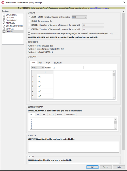
MF6 DISU Package
The Unstructured Discretization (DISU) Package dialog is accessed by double-clicking on the DISU package under a MODFLOW 6 simulation in the Project Explorer. It contains the following sections and options:
- Sections list – A list of sections that can be turned on or off:
- COMMENTS – Turn on to make the COMMENTS section visible.
- OPTIONS – Turn on to make the OPTIONS section visible.
- DIMENSIONS – Turn on to make the DIMENSIONS section visible.
- GRIDDATA – Turn on to make the GRIDDATA section visible.
- CONNECTIONDATA – Turn on to make the CONNECTIONDATA section visible.
- VERTICES – Turn on to make the VERTICES section visible.
- CELL2D – Turn on to make the CELL2D section visible.
- COMMENTS section – Enter general alphanumeric comments. Comments entered here get written at the top of the file, preceded by a '#' symbol.
- OPTIONS section – Options and settings:
- LENGTH_UNITS – This allows for the length units for the model to be specified. Turning it on will activate a drop-down, with the following options:
- "FEET"
- "METERS"
- "CENTIMETERS"
- "UNKNOWN" – The default value if no other one is specified.
- NOGRB – This indicates to deactivate writing of the binary grid file, so there will not be one.
- XORIGIN – This indicates the X-position of the origin used for the model grid vertices (this value is defined by the grid and is not editable). Turning it on will activate a textbox where its value (for the X-position of the lower-left corner of the model grid) will be displayed. This value should be provided in a real-world coordinate system. This value does not affect the model simulation, but is written to the binary grid file so that postprocessors will be able to locate the grid in space. If this value hasn't been set, a default value of 0.0 will be used.
- YORIGIN – This indicates the Y-position of the origin used for the model grid vertices (this value is defined by the grid and is not editable). Turning it on will activate a textbox where its value (for the Y-position of the lower-left corner of the model grid) will be displayed. This value should be provided in a real-world coordinate system. This value does not affect the model simulation, but is written to the binary grid file so that postprocessors will be able to locate the grid in space. If this value hasn't been set, a default value of 0.0 will be used.
- ANGROT – This indicates the counter-clockwise rotation angle (in degrees) of the model grid coordinate system relative to a real-world coordinate system (this value is defined by the grid and is not editable). Turning it on will activate a textbox where its value (for the counter-clockwise rotation angle (in degrees) of the lower-left corner of the model grid) will be displayed. This value does not affect the model simulation, but is written to the binary grid file so that postprocessors will be able to locate the grid in space. If this value hasn't been set, a default value of 0.0 will be used.
- LENGTH_UNITS – This allows for the length units for the model to be specified. Turning it on will activate a drop-down, with the following options:
- DIMENSIONS section – This deals with the DIMENSIONS block.
- Number of nodes (NODES) – This displays the number of cells in the model grid.
- Number of connections and nodes (NJA) – This displays the sum of the number of connections and NODES. When calculating the total number of connections, the connection from one cell to another is considered to be different from the connection between that other cell back to the original. Therefore NJA is equal to the total number of connections, including connections in both directions, and the total number of cells.
- Number of vertices (NVERT) – This displays the total number of (X, Y) vertex pairs used to define the plan-view shape of each cell in the model grid. If this value is unspecified or set to 0, then the VERTICES and CELL2D blocks will not be read, and their sections below will be blank. For most simulations, NVERT should be specified, as well as the accompanying VERTICES and CELL2D blocks. This information is required if in the NPF Package, XT3D or SAVE_SPECIFIC_DISCHARGE have been specified.
- GRIDDATA section – This deals with the GRIDDATA block.
- Define – This allows data within the GRIDDATA section to be defined. When this is inactive, all of the options within a given tab are grayed out. This option is only specifically available in the IDOMAIN tab. In the AREA and BOT tabs, it is not visible but automatically activated so all the options are activated. In the TOP tab, it is not visible but automatically activated, but there are less options to work with.
- Dataset to Array... – This button brings up a Select Dataset dialog, where a single dataset can be selected for use in the GRIDDATA section. This will populate its spreadsheet. This option is grayed out if Define is not turned on. This only appears in the IDOMAIN, AREA, and BOT tabs.
- Drop-down and Constant/Factor – The drop-down in the GRIDDATA section has two options. The option selected will change the nature of the textbox to its right.
- "CONSTANT" – This will change the textbox to the right to be representative of "Constant". If this is selected, the spreadsheet in the GRIDDATA section will be grayed out.
- "ARRAY" – This will change the textbox to the right to be representative of "Factor". If this is selected, the spreadsheet in the GRIDDATA section will not be grayed out, and its cells will be editable.
- TOP – The TOP tab represents the top elevations for each cell in the model grid.
- BOT – The BOT tab represents the bottom elevations for each cell.
- AREA – The AREA tab represents the cell surface areas (in plan view).
- IDOMAIN – The IDOMAIN tab represents the existence status of cells. This is optional to deal with. If it isn't specified, then all model cells exist within the solution. If the value for a cell is 0, the cell does not exist in the simulation. Input and output values will still be read and written for it, but internal to the program, it is excluded from the solution. If the value for a cell is 1, the cell exists in the simulation. If the value for a cell is -1, the cell does not exist in the simulation, however in this case the first existing cell above it will be connected to the first existing cell below it. This type of cell is referred to as a “vertical pass through” cell.
- CONNECTIONDATA section – This deals with the CONNECTIONDATA block. This section is defined by the grid and is not editable.
- IAC – The IAC tab represents the number of connections (plus 1) for each cell. The sum of all IAC entries must be equal to the value of NJA.
- JA – The JA tab represents a list that consists of cell numbers, each followed by all of the cell numbers of the cells that are connected to the relevant cell. The number of values to provide for a cell n is IAC(n). The list is sequentially provided to display from the first to the last cell. The first value in the list must be cell n itself, and the remaining cells must be listed in an increasing order (sorted from lowest number to highest). Note that cells and their connections are only supplied for the GWF cells and their connections to the other GWF cells. To ease readability, for each new cell whose connectivity is subsequently listed, their node number can be expressed as a negative number. The code will later convert the sign to positive.
- IHC – The IHC tab represents an index array that indicates the direction between a node n and all of its m connections. To ease readability, for each new node n, their node number can be expressed as a negative number. The code will later convert the sign to positive. For each IHC value:
- If IHC = 0: Cell n and cell m are connected in the vertical direction. Cell n overlies cell m if the cell number for n is less than m; cell m overlies cell n if the cell number for m is less than n.
- If IHC = 1: Cell n and cell m are connected in the horizontal direction.
- If IHC = 2: Cell n and cell m are connected in the horizontal direction, and the connection is vertically staggered. A vertically staggered connection is one in which a cell is horizontally connected to more than one cell in a horizontal connection.
- CL12 – The CL12 tab represents an array containing connection lengths between the center of cells and the shared face with each of their adjacent cells. To ease readability, for each new cell whose connection lengths are subsequently listed, their node number can be expressed as a negative number. The code will later convert the sign to positive.
- HWVA – The HWVA tab represents a symmetric array with a size the value of NJA. HWVA array entries are the horizontal width perpendicular to flow for horizontal connections, and the vertical area for flow for vertical connections, which means HWVA array values contain both length and area dimensions. HWVA array entries have a one-to-one correspondence with JA array connections and IHC array entries (which specify either a horizontal or vertical connection type). HWVA array entries will be symmetric. If the HWVA value for an n to m connection is not equal to the HWVA value for its corresponding m to n connection, the program will terminate with an error. To ease readability, for each new cell whose connections are subsequently listed, their node number can be expressed as a negative number. The code will later convert the sign to positive.
- ANGLDEGX – The ANGLDEGX tab represents the angle (in degrees) between the horizontal X-axis and the outward normal to the face between a cell and its connecting cells. The angle varies between 0.0 and 360.0 degrees, with 0.0 degrees marking the positive X-axis direction, and 90.0 degrees marking the positive Y-axis direction. ANGLDEGX will only be needed if in the NPF Package, horizontal anisotropy, XT3D, or SAVE_SPECIFIC_DISCHARGE are specified. If these conditions are not met, it will not need to be specified. ANGLDEGX will have a size the value of NJA, values specified for the vertical connections and the diagonal position are not used. Note that ANGLDEGX is read in degrees, which is different from MODFLOW-USG, which used a similar variable (ANGLEX) and read it in radians.
- VERTICES section – This deals with the VERTICES block. This section is defined by the grid and is not editable.
- CELL2D section – This deals with the CELL2D block. This section is defined by the grid and is not editable.
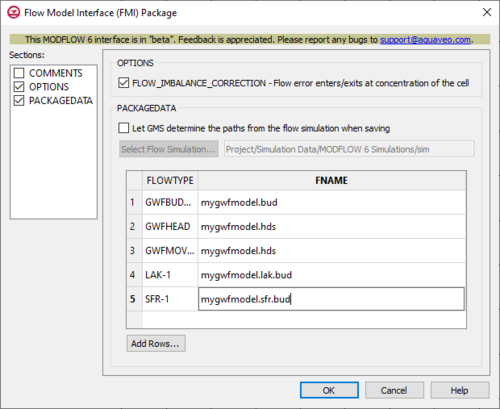
MF6 FMI Package
The Flow Model Interface (FMI) Package dialog is accessed by double-clicking on the FMI package under a MODFLOW 6 simulation in the Project Explorer. It contains the following sections and options:
- Sections list – A list of sections that can be turned on or off:
- COMMENTS – Turn on to make the COMMENTS section visible.
- OPTIONS – Turn on to make the OPTIONS section visible.
- PACKAGEDATA – Turn on to make the PACKAGEDATA section visible.
- COMMENTS section – Enter general alphanumeric comments. Comments entered here get written at the top of the file, preceded by a '#' symbol.
- OPTIONS section – Options and settings:
- FLOW_IMBALANCE_CORRECTION – This indicates to correct for an imbalance in flows by assuming that any residual flow error enters/exits at the concentration of the cell.
- PACKAGEDATA section – This deals with the PACKAGEDATA block.
- Let GMS determine the paths from the flow simulation when saving – Turning this on will gray out the spreadsheet in the PACKAGEDATA section, and activate the Select Flow Simulation... button and its associated textbox.
- Select Flow Simulation... – Clicking this button will bring up the Select Flow Simulation dialog, where a flow simulation can be selected for GMS to use to determine paths when saving. When a file is selected, its address will be displayed in the textbox to the right.
- Add Rows... – This button brings up a Rows to Add dialog, where a number can be specified in the numeric updown to the right of Number of rows to add at bottom. This will help populate the spreadsheet.
- FLOWTYPE – This column represents the FLOWTYPE values, which are either denoted as "GWFBUDGET", "GWFHEAD", "GWFMOVER", or the name of an advanced GWF stress package. If the value is "GWFBUDGET", then its corresponding file will need to be a budget file from a previous GWF Model run. If the value is the name of an advanced GWF stress package, then its corresponding file will need to be a budget file saved by a LAK, SFR, MAW, or UZF Package.
- FNAME – This column represents the FNAME values, which are the names of the files containing flows. If a file is not located in the folder where the program was run, the path to that file should be included.
- Let GMS determine the paths from the flow simulation when saving – Turning this on will gray out the spreadsheet in the PACKAGEDATA section, and activate the Select Flow Simulation... button and its associated textbox.
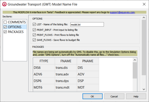
MF6 GWT Package
The Groundwater Transport (GWT) Model Name File dialog is accessed by double-clicking on the GWT model under a MODFLOW 6 simulation in the Project Explorer. It contains the following sections and options:
- Sections list – A list of sections that can be turned on or off:
- COMMENTS – Turn on to make the COMMENTS section visible.
- OPTIONS – Turn on to make the OPTIONS section visible.
- PACKAGES – Turn on to make the PACKAGES section visible.
- COMMENTS section – Enter general alphanumeric comments. Comments entered here get written at the top of the file, preceded by a '#' symbol.
- OPTIONS section – Options and settings:
- LIST – This allows a name for the listing file to be entered.
- PRINT_INPUT – This indicates that the list of input will be printed to the listing file immediately after it is read.
- PRINT_FLOWS – This indicates that the list of flow rates will be printed to the listing file.
- SAVE_FLOWS – This indicates that flow terms will be saved to a budget file.
- PACKAGES section – This deals with the PACKAGES block.
- ftype – This column represents the ftype values, which are the file types of each entry.
- fname – This column represents the fname values, which are the names of the files containing flows.
- pname – This column represents the pname values, which are the Project Explorer item names of the packages (these cannot be changed in the spreadsheet).
MF6 IST Package
The Immobile Storage and Transfer (IST) Package dialog is accessed by double-clicking on the IST package under a MODFLOW 6 simulation in the Project Explorer. It contains the following sections and options:
- Sections list – A list of sections that can be turned on or off:
- COMMENTS – Turn on to make the COMMENTS section visible.
- OPTIONS – Turn on to make the OPTIONS section visible.
- GRIDDATA – Turn on to make the GRIDDATA section visible.
- COMMENTS section – Enter general alphanumeric comments. Comments entered here get written at the top of the file, preceded by a '#' symbol.
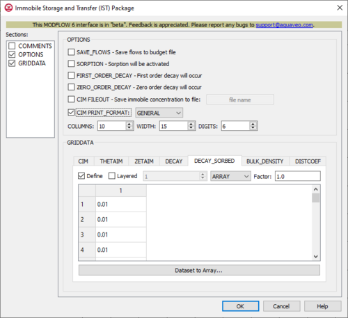
- OPTIONS section – Options and settings:
- SAVE_FLOWS – This indicates that IST flow terms will be saved to a budget file (specified in Output Control with "BUDGET FILEOUT").
- SORPTION – This indicates that sorption will be activated. This requires that BULK_DENSITY and DISTCOEF are specified in the GRIDDATA section.
- FIRST_ORDER_DECAY – This indicates that first-order decay will occur. This requires that DECAY and DECAY_SORBED (if SORPTION has been specified) are specified in the GRIDDATA section.
- ZERO_ORDER_DECAY – This indicates that zero-order decay will occur. This requires that DECAY and DECAY_SORBED (if SORPTION has been specified) are specified in the GRIDDATA section.
- CIM FILEOUT – This allows immobile concentrations to be saved to a specifically defined listing file.
- CIM PRINT_FORMAT – This allows the format that will be used for printing the immobile concentrations to the listing file to be specified. This uses a drop-down that is grayed out until CIM PRINT_FORMAT is specified. The drop-down options are:
- "EXPONENTIAL"
- "FIXED"
- "GENERAL"
- "SCIENTIFIC"
- COLUMNS – A numeric updown that can be used to set the number of columns for printing. This will be grayed out until CIM PRINT_FORMAT is specified.
- WIDTH – A numeric updown that can be used to set the number of the width for printing. This will be grayed out until CIM PRINT_FORMAT is specified.
- DIGITS – A numeric updown that can be used to set the number of digits for printing. This will be grayed out until CIM PRINT_FORMAT is specified.
- GRIDDATA section – This deals with the GRIDDATA block.
- Define – This allows data within the GRIDDATA section to be defined. When this is inactive, all of the options within a given tab are grayed out. This option is only specifically available in the CIM, DECAY, and DECAY_SORBED tabs. In the THETAIM, ZETAIM, BULK_DENSITY, and DISTCOEF tabs, it is not visible but automatically activated so all the options are activated.
- Dataset to Array... – This button brings up a Select Dataset dialog, where a single dataset can be selected for use in the GRIDDATA section. This will populate its spreadsheet. This option is grayed out if Define is not turned on.
- Layered – When this is active, a numeric updown for the layers will become available.
- Drop-down and Constant/Factor – The drop-down in the GRIDDATA section has two options. The option selected will change the nature of the textbox to its right.
- "CONSTANT" – This will change the textbox to the right to be representative of "Constant". If this is selected, the spreadsheet in the GRIDDATA section will be grayed out.
- "ARRAY" – This will change the textbox to the right to be representative of "Factor". If this is selected, the spreadsheet in the GRIDDATA section will not be grayed out, and its cells will be editable.
- CIM – The CIM tab represents the initial concentrations of the immobile domain in mass per length cubed. If a value is not specified, then it will automatically be assumed to be 0.
- THETAIM – The THETAIM tab represents the porosities of the immobile domain specified as the volume of immobile pore space per total volume (dimensionless).
- ZETAIM – The ZETAIM tab represents the mass transfer rate coefficients between the mobile and immobile domains (in dimension of per time).
- DECAY – The DECAY tab represents the rate coefficients for first/zero-order decay for the aqueous phase of the immobile domain. Negative values indicate solute production. For first-order decay, the dimensions of DECAY is one over time. For zero-order decay, the dimensions of DECAY is mass per length cubed per time. If neither FIRST_ORDER_DECAY nor ZERO_ORDER_DECAY are specified, then DECAY will have no impact on simulation results.
- DECAY_SORBED – The DECAY_SORBED tab represents the rate coefficients for first/zero-order decay for the sorbed phase of the immobile domain. Negative values indicate solute production. For first-order decay, the dimension of DECAY_SORBED is one over time. For zero-order decay, the dimensions of DECAY_SORBED is mass of solute per mass of aquifer per time. If DECAY_SORBED is not specified, but both DECAY and SORPTION are active, the sorbed decay rate will be set to the same value as the aqueous decay rate. If SORPTION hasn't been specified and neither FIRST_ORDER_DECAY nor ZERO_ORDER_DECAY have been specified, then DECAY_SORBED will have no impact on simulation results.
- BULK_DENSITY – The BULK_DENSITY tab represents the bulk densities of the aquifer in mass per length cubed. If SORPTION hasn't been specified, then BULK_DENSITY will have no impact on simulation results.
- DISTCOEF – The DISTCOEF tab represents the distribution coefficients for the equilibrium-controlled linear sorption isotherm in dimensions of length cubed per mass. If SORPTION hasn't been specified, then DISTCOEF will have no impact on simulation results.
MF6 LKT Package
The Lake Transport (LKT) Package dialog is accessed by double-clicking on the LKT package under a MODFLOW 6 simulation in the Project Explorer. It contains the following sections and options:
- Sections list – A list of sections that can be turned on or off:
- COMMENTS – Turn on to make the COMMENTS section visible.
- OPTIONS – Turn on to make the OPTIONS section visible.
- DATA – Turn on to make the DATA section visible.
- COMMENTS section – Enter general alphanumeric comments. Comments entered here get written at the top of the file, preceded by a '#' symbol.
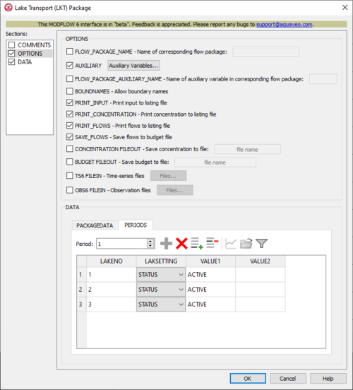
- OPTIONS section – Options and settings:
- FLOW_PACKAGE_NAME – This allows the name of the corresponding flow package to be specified. Turning this on will activate a textbox to the right where this can be entered. If this isn't specified, the corresponding flow package will need to have the same name as this advanced transport package (the name associated with this package in the GWT name file).
- AUXILIARY – This allows an array of one or more auxiliary variables to be named. There are no limits to the number of auxiliary variables that can be provided, but subsequent blocks will require data for each of the auxiliary variables that are defined. Turning this on will activate an Auxiliary Variables... button. Clicking the button will bring up an Auxiliary Variables dialog. The following options can be used to help develop the auxiliary variables:
- Insert Row – This will insert a new row at the current location.
- Add Row – This will add a new row at the bottom.
- Delete Row – This will delete the currently selected row.
- Move Up – This will move the currently selected row up a row.
- Move Down – This will move the currently selected row down a row.
- FLOW_PACKAGE_AUXILIARY_NAME – This allows the name of an auxiliary variable in the corresponding flow package to be specified. Turning this on will activate a textbox to the right where this can be entered. If this is specified, then this advanced transport package's simulated concentrations will be copied into the auxiliary variable specified with the entered name. If the flow package does not have an auxiliary variable with this name, the program will terminate with an error. This option will have no affect if the flows for this advanced transport package are read from a file.
- BOUNDNAMES – This indicates that boundary names are allowed to be provided with the list of lake cells. This will add the BOUNDNAME column to the spreadsheet in the DATA section.
- PRINT_INPUT – This indicates that the list of lake information input will be printed to the listing file immediately after it is read.
- PRINT_CONCENTRATION – This indicates that the list of lake concentration will be printed to the listing file, for every stress period where “HEAD PRINT” has been specified in Output Control. If PRINT_CONCENTRATION has been specified when there is no Output Control option, then they will be printed for the last time step of each stress period.
- PRINT_FLOWS – This indicates that the list of lake flow rates will be printed to the listing file, for every stress period time step where “BUDGET PRINT” has been specified in Output Control. If PRINT_FLOWS has been specified when there is no Output Control option, then they will be printed for the last time step of each stress period.
- SAVE_FLOWS – This indicates that lake flow terms will be saved to a budget file (specified in Output Control with "BUDGET FILEOUT").
- CONCENTRATION FILEOUT – This allows concentration information to be saved to a specifically defined binary output file.
- BUDGET FILEOUT – This allows budget information to be saved to a specifically defined binary output file.
- TS6 FILEIN – This allows time series files to be used as input to assign time-varying values. Specifying this option will allow a Files... button to its right to be clicked. Doing so will bring up a Files dialog. In this dialog, a spreadsheet can be filled in that has two columns. The following options can be used to help develop the spreadsheet:
- Insert Row – This will insert a new row at the current location.
- Add Row – This will add a new row at the bottom.
- Delete Row – This will delete the currently selected row.
- Move Up – This will move the currently selected row up a row.
- Move Down – This will move the currently selected row down a row.
- OBS6 FILEIN – This allows observations files to be used as input. Specifying this option will allow a Files... button to its right to be clicked. Doing so will bring up a Files dialog. In this dialog, a spreadsheet can be filled in that has two columns. The first column allows filenames to be specified. The second column has an Edit... button relating to the file specified. The following options can be used to help develop the spreadsheet:
- Insert Row – This will insert a new row at the current location.
- Add Row – This will add a new row at the bottom.
- Delete Row – This will delete the currently selected row.
- Move Up – This will move the currently selected row up a row.
- Move Down – This will move the currently selected row down a row.
- DATA section – This deals with the DATA block.
- PACKAGEDATA –
- Set Up From LAK6 Package – This button allows for PACKAGEDATA to be set up from an already existing LAK6 Package. If one cannot be found, a warning dialog will come up saying so.
- Add Rows... – This button brings up a Rows to Add dialog, where a number can be specified to the right of Number of rows to add at bottom. This will help populate the spreadsheet.
- LAKENO – This column represents the LAKENO integer values, which define the lake numbers associated with the PACKAGEDATA data. These values must be greater than zero and less than or equal to the separately defined NLAKES value. If lake information has not been specified for every lake or information for a lake has been specified more than once, the program will terminate with an error.
- STRT – This column represents the STRT real values, which define the starting concentration for the lakes.
- AUX – These columns represent the values of the auxiliary variables for each lake, which previously may have been created if the AUXILIARY option was set. There will need to be values for the auxiliary variables for each lake. If time series files are used as input, entering a time series name instead of a numeric value can allow for values to be obtained from a time series.
- BOUNDNAME – This column represents the names of the lake cells, and will appear if the BOUNDNAMES option was set. BOUNDNAME values are ASCII character variables that can contain as many as 40 characters. If a BOUNDNAME value contains spaces within it, then the entire name will have to be enclosed within single quotes.
- PERIODS –
- Period – A numeric updown can be used to enter which period is being examined in the spreadsheet.
- Define Period – This button will allow a period to be defined. This will be active when no period has yet been defined, and it may gray out once one has been created.
- Delete Period – This button will delete the selected period. A dialog warning will come up first asking the user to confirm their decision to delete the period.
- Add Rows – This button will bring up an Add Stresses dialog. The following options can be used to help in adding the stresses:
- Columns and Values – Numeric updowns, drop-downs, and textboxes can be used to enter the values for their relevant columns for all the new stresses. These may include columns that are not actually present in the spreadsheet.
- Number of rows to add – A numeric updown can be used to enter the number of rows that will be added to the spreadsheet.
- Add to – There are two different options, only one of which can be selected at a time.
- All defined periods – These stresses will be added to all the periods that have been defined.
- Only this period – These stresses will be added only to the currently selected period.
- Delete Rows – This button will delete all of the stresses. A dialog warning will come up first asking the user to confirm their decision to delete the stresses. The dialog will also give them the option to either Delete From All Periods or Delete From Just This Period.
- Plot All Periods – This will allow the user to plot all the periods that have been defined.
- Open Time Series – This will allow the user to open a time series file.
- Filter on Selected Cells – ???
- LAKENO – This column represents the LAKENO integer values, which define the lake numbers associated with the PERIOD data. These values must be greater than zero and less than or equal to the separately defined NLAKES value.
- LAKSETTING – This column represents the LAKSETTING keywords, which can be used to start LAKSETTING strings (lines of information parsed into a keyword and values). These are used to assign the concentration associated with the corresponding flow terms. Concentrations cannot be specified for all flow terms (ex. The Lake Package supports a "WITHDRAWAL" flow term. If this is active, water will be withdrawn from the lake at its calculated concentration.). These keywords are assigned in a drop-down, which can be selected to one of the following options:
- "STATUS" – This keyword option is used to define lake status. The STATUS options are:
- "ACTIVE" – The default value is "ACTIVE", which means the concentration will be calculated for the lake.
- "INACTIVE" – If the value has been set to "INACTIVE", then there will be no solute mass fluxes into/out of the lake and the inactive value will be written for the lake concentration.
- "CONSTANT" – If the value has been set to "CONSTANT", then the concentration for the lake will be fixed at the user-specified value.
- "CONCENTRATION" – This keyword option uses a real/character value to define the concentration for the lake. The specified value will only be applied for constant concentration lakes. If time series files are used as input, entering a time series name instead of a numeric value can allow for values to be obtained from a time series.
- "RAINFALL" – This keyword option uses a real/character value to define the rainfall solute concentration (ML-3) for the lake. If time series files are used as input, entering a time series name instead of a numeric value can allow for values to be obtained from a time series.
- "EVAPORATION" – This keyword option uses a real/character value to define the concentration of evaporated water (ML-3) for the lake. When this value is larger than the simulated concentration in the lake, then evaporated water will be removed at the same concentration as the lake. If time series files are used as input, entering a time series name instead of a numeric value can allow for values to be obtained from a time series.
- "RUNOFF" – This keyword option uses a real/character value to define the concentration of runoff (ML-3) for the lake. This value will need to be greater than or equal to zero. If time series files are used as input, entering a time series name instead of a numeric value can allow for values to be obtained from a time series.
- "AUXILIARY" – This keyword option is used to specify auxiliary variables, and will require two values to be properly used. The first value will be for the AUXNAME, the name for the auxiliary variable that will be assigned an AUXVAL. This AUXNAME will need to match one of the names that was previously defined for the auxiliary variables in the OPTIONS section. If it does not, the entered data will be ignored. The second value will be for the AUXVAL, the value for the auxiliary variable that was named. If time series files are used as input, entering a time series name instead of a numeric value can allow for values to be obtained from a time series.
- "STATUS" – This keyword option is used to define lake status. The STATUS options are:
- VALUE1 – This column is for the first value following the keyword specified in the LAKSETTING column. For most keywords, only this column will be needed.
- VALUE2 – This column is for the second value following the keyword specified in the LAKSETTING column. Only "AUXILIARY" requires this, as the first value will be an AUXNAME and the second value will be an AUXVAL.
- PACKAGEDATA –
MF6 MST Package
The Mobile Storage and Transfer (MST) Package dialog is accessed by double-clicking on the MST package under a MODFLOW 6 simulation in the Project Explorer. It contains the following sections and options:
- Sections list – A list of sections that can be turned on or off:
- COMMENTS – Turn on to make the COMMENTS section visible.
- OPTIONS – Turn on to make the OPTIONS section visible.
- GRIDDATA – Turn on to make the GRIDDATA section visible.
- COMMENTS section – Enter general alphanumeric comments. Comments entered here get written at the top of the file, preceded by a '#' symbol.
- OPTIONS section – Options and settings:
- SAVE_FLOWS – This indicates that MST flow terms will be saved to a budget file (specified in Output Control with "BUDGET FILEOUT").
- FIRST_ORDER_DECAY – This indicates that first-order decay will occur. This requires that DECAY and DECAY_SORBED (if SORPTION has been specified) are specified in the GRIDDATA section.
- ZERO_ORDER_DECAY – This indicates that zero-order decay will occur. This requires that DECAY and DECAY_SORBED (if SORPTION has been specified) are specified in the GRIDDATA section.
- SORPTION – This indicates that sorption will be activated. This requires that BULK_DENSITY and DISTCOEF are specified in the GRIDDATA section. This will also activate a drop-down where the type of sorption can be chosen, from the following options:
- "LINEAR"
- "FREUNDLICH"
- "LANGMUIR"
- GRIDDATA section – This deals with the GRIDDATA block.
- Define – This allows data within the GRIDDATA section to be defined. When this is inactive, all of the options within a given tab are grayed out. This option is specifically available in all of the tabs except for the POROSITY tab. In the POROSITY tab, it is not visible but automatically activated so all the options are activated.
- Dataset to Array... – This button brings up a Select Dataset dialog, where a single dataset can be selected for use in the GRIDDATA section. This will populate its spreadsheet. This option is grayed out if Define is not turned on.
- Layered – When this is active, a numeric updown for the layers will become available.
- Drop-down and Constant/Factor – The drop-down in the GRIDDATA section has two options. The option selected will change the nature of the textbox to its right.
- "CONSTANT" – This will change the textbox to the right to be representative of "Constant". If this is selected, the spreadsheet in the GRIDDATA section will be grayed out.
- "ARRAY" – This will change the textbox to the right to be representative of "Factor". If this is selected, the spreadsheet in the GRIDDATA section will not be grayed out, and its cells will be editable.
- POROSITY – The POROSITY tab represents the aquifer porosities.
- DECAY – The DECAY tab represents the rate coefficients for first/zero-order decay for the aqueous phase of the mobile domain. Negative values indicate solute production. For first-order decay, the dimensions of DECAY is one over time. For zero-order decay, the dimensions of DECAY is mass per length cubed per time. If neither FIRST_ORDER_DECAY nor ZERO_ORDER_DECAY are specified, then DECAY will have no impact on simulation results.
- DECAY_SORBED – The DECAY_SORBED tab represents the rate coefficients for first/zero-order decay for the sorbed phase of the mobile domain. Negative values indicate solute production. For first-order decay, the dimension of DECAY_SORBED is one over time. For zero-order decay, the dimensions of DECAY_SORBED is mass of solute per mass of aquifer per time. If DECAY_SORBED is not specified, but both DECAY and SORPTION are active, the sorbed decay rate will be set to the same value as the aqueous decay rate. If SORPTION hasn't been specified and neither FIRST_ORDER_DECAY nor ZERO_ORDER_DECAY have been specified, then DECAY_SORBED will have no impact on simulation results.
- BULK_DENSITY – The BULK_DENSITY tab represents the bulk densities of the aquifer in mass per length cubed. If SORPTION hasn't been specified, then BULK_DENSITY will not be required.
- DISTCOEF – The DISTCOEF tab represents the distribution coefficients for the equilibrium-controlled linear sorption isotherm in dimensions of length cubed per mass. If SORPTION hasn't been specified, then DISTCOEF will not be required.
- SP2 – ???
MF6 MVT Package
The Mover Transport (MVT) Package dialog is accessed by double-clicking on the MVT package under a MODFLOW 6 simulation in the Project Explorer. It contains the following sections and options:
- Sections list – A list of sections that can be turned on or off:
- COMMENTS – Turn on to make the COMMENTS section visible.
- OPTIONS – Turn on to make the OPTIONS section visible.
- COMMENTS section – Enter general alphanumeric comments. Comments entered here get written at the top of the file, preceded by a '#' symbol.
- OPTIONS section – Options and settings:
- PRINT_INPUT
- PRINT_FLOWS
- SAVE_FLOWS
- BUDGET FILEOUT
MF6 MWT Package
The Multi-Aquifer Well Transport (MWT) Package dialog is accessed by double-clicking on the MWT package under a MODFLOW 6 simulation in the Project Explorer. It contains the following sections and options:
- Sections list – A list of sections that can be turned on or off:
- COMMENTS – Turn on to make the COMMENTS section visible.
- OPTIONS – Turn on to make the OPTIONS section visible.
- DATA – Turn on to make the DATA section visible.
- COMMENTS section – Enter general alphanumeric comments. Comments entered here get written at the top of the file, preceded by a '#' symbol.
- OPTIONS section – Options and settings:
- FLOW_PACKAGE_NAME
- AUXILIARY
- FLOW_PACKAGE_AUXILIARY_NAME
- BOUNDNAMES
- PRINT_INPUT
- PRINT_CONCENTRATION
- PRINT_FLOWS
- SAVE_FLOWS
- CONCENTRATION FILEOUT
- BUDGET FILEOUT
- TS6 FILEIN
- OBS6 FILEIN
- DATA section – This deals with the DATA block.
- PACKAGEDATA
- PERIODS
MF6 SFT Package
The Streamflow Transport (SFT) Package dialog is accessed by double-clicking on the SFT package under a MODFLOW 6 simulation in the Project Explorer. It contains the following sections and options:
- Sections list – A list of sections that can be turned on or off:
- COMMENTS – Turn on to make the COMMENTS section visible.
- OPTIONS – Turn on to make the OPTIONS section visible.
- DATA – Turn on to make the DATA section visible.
- COMMENTS section – Enter general alphanumeric comments. Comments entered here get written at the top of the file, preceded by a '#' symbol.
- OPTIONS section – Options and settings:
- FLOW_PACKAGE_NAME
- AUXILIARY
- FLOW_PACKAGE_AUXILIARY_NAME
- BOUNDNAMES
- PRINT_INPUT
- PRINT_CONCENTRATION
- PRINT_FLOWS
- SAVE_FLOWS
- CONCENTRATION FILEOUT
- BUDGET FILEOUT
- TS6 FILEIN
- OBS6 FILEIN
- DATA section – This deals with the DATA block.
- PACKAGEDATA
- PERIODS
MF6 SRC Package
The Mass Source Loading (SRC) Package dialog is accessed by double-clicking on the SRC package under a MODFLOW 6 simulation in the Project Explorer. It contains the following sections and options:
- Sections list – A list of sections that can be turned on or off:
- COMMENTS – Turn on to make the COMMENTS section visible.
- OPTIONS – Turn on to make the OPTIONS section visible.
- PERIODS – Turn on to make the PERIODS section visible.
- COMMENTS section – Enter general alphanumeric comments. Comments entered here get written at the top of the file, preceded by a '#' symbol.
- OPTIONS section – Options and settings:
- AUXILIARY
- AUXMULTNAME
- BOUNDNAMES
- PRINT_INPUT
- PRINT_FLOWS
- SAVE_FLOWS
- TS6 FILEIN
- OBS6 FILEIN
- PERIODS section – This deals with the PERIODS block.
- Period
- Define Period
- Delete Period
- Add Rows
- Delete Rows
- Plot All Periods
- Open Time Series
- Filter on Selected Cells
- LAY
- ROW
MF6 SSM Package
The Source and Sink Mixing (SSM) Package dialog is accessed by double-clicking on the SSM package under a MODFLOW 6 simulation in the Project Explorer. It contains the following sections and options:
- Sections list – A list of sections that can be turned on or off:
- COMMENTS – Turn on to make the COMMENTS section visible.
- OPTIONS – Turn on to make the OPTIONS section visible.
- SOURCES – Turn on to make the SOURCES section visible.
- COMMENTS section – Enter general alphanumeric comments. Comments entered here get written at the top of the file, preceded by a '#' symbol.
- OPTIONS section – Options and settings:
- PRINT_FLOWS
- SAVE_FLOWS
- SOURCES section – This deals with the SOURCES block.
- Set Up From Flow Model
- Add Rows...
- PNAME
- SRCTYPE
MF6 UZT Package
The Unsaturated Zone Transport (UZT) Package dialog is accessed by double-clicking on the UZT package under a MODFLOW 6 simulation in the Project Explorer. It contains the following sections and options:
- Sections list – A list of sections that can be turned on or off:
- COMMENTS – Turn on to make the COMMENTS section visible.
- OPTIONS – Turn on to make the OPTIONS section visible.
- DATA – Turn on to make the DATA section visible.
- COMMENTS section – Enter general alphanumeric comments. Comments entered here get written at the top of the file, preceded by a '#' symbol.
- OPTIONS section – Options and settings:
- FLOW_PACKAGE_NAME
- AUXILIARY
- FLOW_PACKAGE_AUXILIARY_NAME
- BOUNDNAMES
- PRINT_INPUT
- PRINT_CONCENTRATION
- PRINT_FLOWS
- SAVE_FLOWS
- CONCENTRATION FILEOUT
- BUDGET FILEOUT
- TS6 FILEIN
- OBS6 FILEIN
- DATA section – This deals with the DATA block.
- PACKAGEDATA
- PERIODS
Arrays to Datasets
GWF-GWF Exchange
The Groundwater Flow (GWF) Exchange dialog is accessed by double-clicking on the GWF-GWF package under a MODFLOW 6 simulation in the Project Explorer. It contains the following sections and options:
- Sections list – A list of sections that can be turned on or off:
- COMMENTS – Turn on to make the COMMENTS section visible.
- OPTIONS – Turn on to make the OPTIONS section visible.
- EXCHANGEDATA – Turn on to make the EXCHANGEDATA section visible.
- COMMENTS section – Enter general alphanumeric comments. Comments entered here get written at the top of the file, preceded by a '#' symbol.
- OPTIONS section – Options and settings:
- AUXILIARY
- PRINT_INPUT
- PRINT_FLOWS
- SAVE_FLOWS
- CELL_AVERAGING
- VARIABLECV
- NEWTON
- GNC6 FILEIN
- MVR6 FILEIN
- OBS6 FILEIN
- EXCHANGEDATA section – This deals with the EXCHANGEDATA block.
- Add Rows...
- LAYM1
- ROWM1
- COLM1
- LAYM2
- ROWM2
- COLM2
- IHC
- CL1
- CL2
- HWVA
GWF-GWT Exchange
The Groundwater Transport (GWT) Exchange dialog is accessed by double-clicking on the GWF-GWT package under a MODFLOW 6 simulation in the Project Explorer. It contains the following sections and options:
- Sections list – A list of sections that can be turned on or off:
- COMMENTS – Turn on to make the COMMENTS section visible.
- COMMENTS section – Enter general alphanumeric comments. Comments entered here get written at the top of the file, preceded by a '#' symbol.

