Template:Convert 3D Data to 2D Data
The Convert 3D Data to 2D Data tool is used to convert 3D cell data to a 2D UGrid with datasets. The user selects a 3D cell dataset as input to the tool (the dataset may have multiple time steps). Then the user may choose to output multiple datasets from the tool; the following datasets may be computed by the tool: highest active value, average, maximum, minimum, value for each layer. The 3D UGrid cells are organized into columns of cells to compute the various output datasets. Examples follow that explain how the tool works for different types of UGrids.
This tool will only work on UGrids that are made up of 3D cells and those cells must all be prisms (the side faces of the cells must be vertical). Further, the grid must have layers assigned to the cells. The tool will return an error if any of these conditions are not met.
Input parameters
- Cell dataset – The input 3D dataset that will be converted to 2D datasets
- Name of the output grid – Name for the newly created 2D UGrid. If this value is left blank then the name of the output grid will be set to be the name of the input cell dataset.
- Compute highest active cell in column – Option to output a 2D dataset where the value will come from the highest active cell in the 3D column of cells.
- Compute average value in column – Option to output a 2D dataset of the average value in the 3D column of cells.
- Compute maximum value in column – Option to output a 2D dataset of the maximum value in the 3D column of cells.
- Compute minimum value in column – Option to output a 2D dataset of the minimum value in the 3D column of cells.
- Compute value for each layer in column – Option to output 2D datasets of the value for each layer in the 3D column of cells.
Output parameters
- The output is a 2D UGrid and datasets.
Current location in Toolbox
UGrids/Convert 3D Data to 2D Data
Examples
Files for example 1 and example 3 can be downloaded here. (Include a link to download these files.)
Example 1
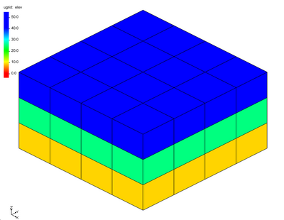
The first example is a simple structured 3D Grid. The grid is made up of 4 rows, 4 columns, and 3 layers.
The dataset “elev” has constant values for each layer of the grid: layer 1 – 41.6, layer 2 – 25.0, and layer 3 – 8.3. Running the tool on this dataset produces the following 2D UGrid and datasets.
In this example the datasets are straight forward.
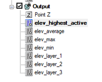
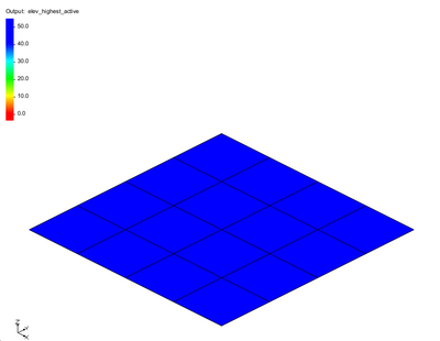
The "elev_highest_active" creates a dataset with values from the top of the 3D UGrid. All of the values are 41.6. The "elev_average" dataset gives the average value in each cell column and in this case that will match the values from layer 2 of the 3D UGrid (25.0). The elev_max dataset matches the values of the top layer of the 3D UGrid (41.6). The "elev_min" dataset matches the values from the bottom layer of the 3D UGrid (8.3). The "elev_layer_1", "elev_layer_2", and "elev_layer_3" match the values from the respective layer of the 3D UGrid.
Example 2
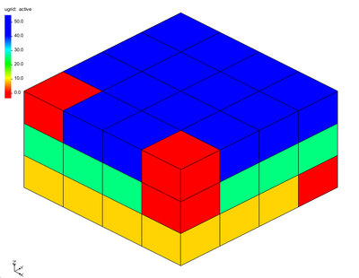
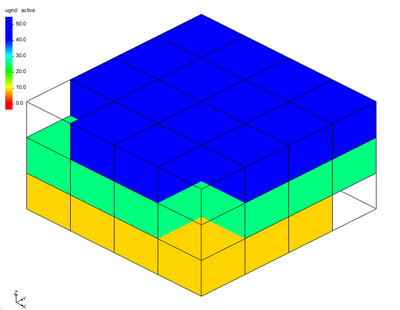
The second example is the same 3D Grid from example 1 except in this case the 3D dataset has activity. That is to say, some of the values in the dataset are considered inactive. The cells with inactive values are shown in red in the following figure.
Typically, these values are not contoured on the 3D UGrid.
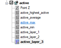
When the tool runs with this example the following datasets are created. First, examine the layer datasets and notice the effect that activity has on the created datasets.
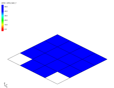
The "active_layer_1" dataset shows the 2 cells with inactive values.
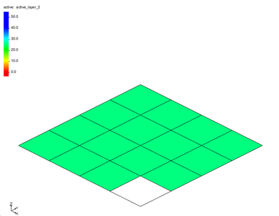
The "active_layer_2" dataset show the 1 cell with an inactive value.
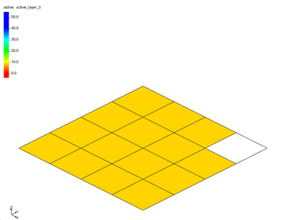
The "active_layer_3" dataset shows the 1 cell with an inactive value.
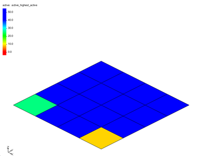
The "active_highest_active" has values from 2 of the lower layers in the 3D UGrid.
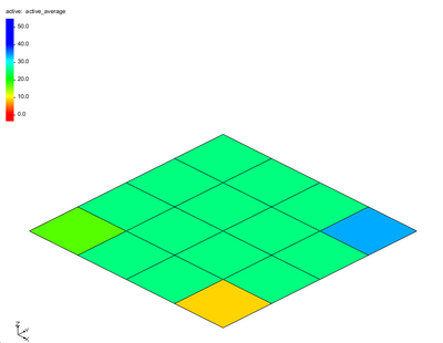
The "active_average" has 3 values that are affected by the dataset activity. The "active_maximum" and "active_minimum" datasets are similar to the "active_average".
Example 3
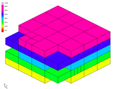
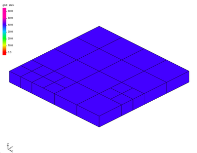
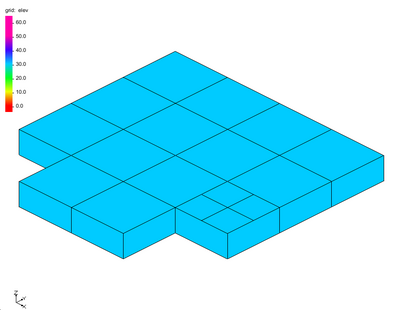
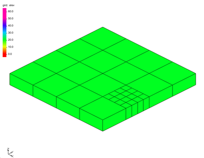
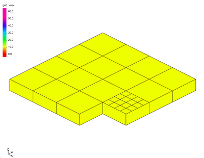
The third example is a 3D UGrid with variable number of cells per layer and variable refinement in each layer. A figure of the entire grid is shown, followed by figures of individual layers.
Layer 1 of the 3D UGrid:
Layer 2 of the 3D UGrid:
Layer 3 of the 3D UGrid:
Layer 4 of the 3D UGrid:
Layer 5 of the 3D UGrid:
When the tool is run with this example the following datasets are created.
The next figure shows the resulting 2D UGrid with the elev_highest_active dataset contoured.
Notice that the 2D cells are defined by the smallest 3D cells in any column. The 2 cells that are not pink have values that came from layer 2 of the 3D Grid. The elev_average, elev_maximum, elev_minimum are computed in a straight forward manner and are not shown here. The elev_layer datasets are shown next. Notice that some layer datasets have inactive values because there were no cells defined in those cell columns.
The elev_layer_1 dataset.
The elev_layer_2 dataset.
The elev_layer_3 dataset.
The elev_layer_4 dataset.
The elev_layer_4 dataset.
Example 4
The fourth example uses the same 3D UGrid as example 3 and the dataset now includes activity. The orange cells in the grid have a value of 5. The red cells have inactive dataset values.
Layer 2 values for 3D UGrid.
When the tool is executed the following results are generated from the tool.
The active_highest_active dataset result.
The active_layer_1 dataset.
The active_layer_2 dataset.
The active_layer_3 dataset.
The active_layer_4 dataset.
The active_layer_5 dataset.
Example 5
The fifth example is a voronoi 3D UGrid. This grid has a variable number of cells in each layer. This example comes from the MODFLOW-USG Complex Stratigraphy tutorial.
Layer 2 of 3D UGrid
Layer 3 of 3D UGrid
Layer 4 of 3D UGrid
Layer 5 of 3D UGrid. When the tool is run the following figure shows the output 2D UGrid.
