WMS:CE-QUAL-W2 Bathymetry

Laterally Averaged Finite Difference Grids

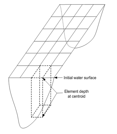
Most hydrodynamic models are depth-averaged, meaning that the numerical mesh (finite difference or finite element) is oriented in the x-y plane with each element representing a vertical column, or an average depth, of the domain being modeled. Tools for generating depth-averaged numerical models have been well developed because of the number of applications (Fugal, 2000; Thibodeaux, 1992; Gaspar et. al., 1994). Average depths for each element are determined by estimating an initial water surface level and then calculating the depth at each element centroid using bathymetric elevation data. The typical process requires the user to define a spatial domain of the model and then appropriately fill the regions with finite elements (quadrilaterals and/or triangles). Finally, a depth for each column is determined by calculating the difference between the assumed or starting water surface elevation of the element and the elevation determined from data gathered that describes the underlying bathymetry (see Figure 1).

Figure 1: Depth calculation for a depth-averaged finite difference grid.

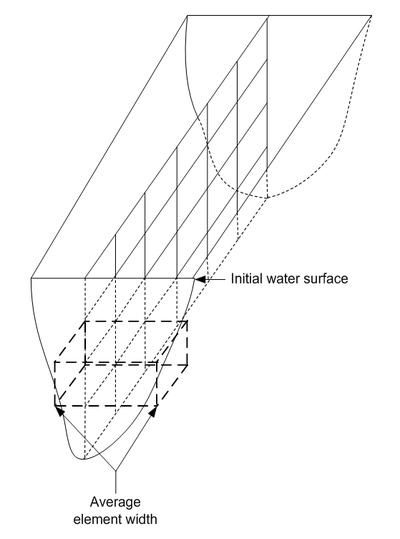
A major limitation of depth-averaged models is that they do not represent vertical variations well. For example, velocities computed using such a model do not account for variations that may occur between the top and bottom of the model since a single, average, value for each vertical column is computed. On the other hand, a laterally averaged numerical model better represents vertical variations, an important aspect of deeper water bodies such as lakes and reservoirs. However, in order to develop a laterally averaged numerical model an average width for each element must be determined. Unlike the depth-averaged models it is not possible to assume some initial “bank location” and then estimate the width to each element. Instead the bathymetry describing the shoreline elevations on either side of the model must be known so that a width at each element can be estimated as illustrated in Figure 2.

Figure 2: Width calculation for a laterally-averaged finite difference grid.

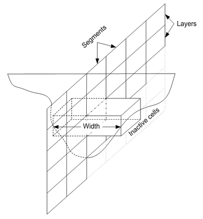
To develop the geometric representation for such models, discretization along the length and depth of the model must first be determined. In CE-QUAL-W2, segment lengths are determined from the spatial orientation of the water body. Tributary inflows, widening/narrowing of the water body and sampling or computational points are all indicators of how to divide the model up along its length into segments. Layer depths are generally a function of the sensitivity, or gradient of the vertical variations of the variables being analyzed (i.e. temperature, phosphorous, dissolved oxygen, etc.). The higher the gradient the smaller the element heights should be. Once lengths and heights are determined a finite difference grid representing the profile of the water body can be constructed as shown in Figure 3. Cells are inactive if their centroid elevation drops below the bottom elevation of the water body. The final dimension required for the grid geometry of the model is an average width as illustrated in Figure 3.

Figure 3: Finite difference grid representation of a CE-QUAL W2 model.

Average widths are generally determined from the water body’s bathymetric data. This is the most difficult task in preparing the model geometry because each element width is unique (i.e. separate measurements required).

Estimating Average Widths

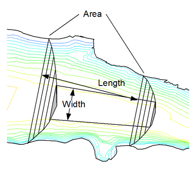
Widths are generally calculated from contours or sediment survey transects (cross sections) of the model bathymetry. In the case of contours a width is calculated by first determining the depth at the centroid of the segment at the layer and then measuring the distance at either side of the segment centerline to the contour with that elevation as shown in Figure 4.

Figure 4: Measuring element widths from contours.

Alternatively, transects at both ends of the element segment can be drawn until they intersect the contour at the centroid elevation. The area bounded by these contours and the segment ends determines a width calculated by dividing the area by the segment length. Even with excellent computer aided drawing (CAD) tools this is a tedious process and has prevented widespread use of such models, even though they are superior for problems in which vertical variations are important.

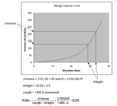
Most existing reservoirs have volume-elevation curves and/or area-elevation curves (referred to throughout the rest of this paper as storage capacity curves) as part of their design. Such curves allow managers to quickly determine storage volumes or surface areas for a given water surface elevation. If a storage capacity curve for each of the model segments could be generated, computing element widths at the different layers within the segment would be straightforward and easy to automate in a computer algorithm. Once a volume is determined for an element centroidal depth the average width is easily computed from the three known quantities:

$Width={\frac {Volume}{(Length)(Height)}}$

Figure 5 illustrates how volumes and a resulting segment width are determined for any given depth.

Figure 5: Calculation of width from incremental volumes between two reservoir heights.

The key then to automating a process for developing geometric properties from bathymetric data is to develop a separate storage capacity curve for each of the model segments.

Storage Capacity Curve Generation From TIN

Triangulated Irregular Networks (TINs) are used by many programs to develop contours and compute other surface properties from scattered xyz elevation data (Lee and Schacter 1980, Watson 1981). A TIN is created by triangulating the xyz data points into a series of non-overlapping triangles which collectively form a piece-wise linear approximation of the surface. For CE-QUAL-W2 models, a TIN is used to compute a storage capacity curve for each segment.

Because a TIN is a piecewise linear representation of a surface, isolines can easily be computed for any given elevation. By bounding the TIN with the segment beginning and ending transects the area for any given contour elevation can be determined automatically. Any elevation interval can be chosen, but since the computations are automated with a computer algorithm a large number of areas (i.e. a small interval) for given elevations can be computed in a relatively short period of time generating a smooth elevation vs. area curve for the segment.

In order to compare with existing data typically developed during construction of a reservoir, a storage capacity curve (elevation vs. volume) is also determined using the conic method as outlined by the U.S. Army Corps of Engineers (HEC-1 1991). In the conic method incremental volumes between areas at elevations E1 and E2 (see Figure 6) are computed using the following equation:

$DeltaV_{1}2={\frac {h}{3}}(A_{1}+A_{2}+sqrt(A_{1}A_{2}))$