SMS:Computed vs. Observed Data Plot: Difference between revisions
No edit summary |
|||
| Line 19: | Line 19: | ||
If a plot will not generate or does not display significant data, it's possible that the conditions for the plot have not been set up correctly. To get a meaningful plot, take the following into account: | If a plot will not generate or does not display significant data, it's possible that the conditions for the plot have not been set up correctly. To get a meaningful plot, take the following into account: | ||
* This plot requires an observation coverage with feature points included that have observation data from the field. | * This plot requires an observation coverage with feature points included that have observation data from the field. | ||
* This plot requires a simulation with calculated data of the same type of data as the observation coverage (velocity, for example). If the simulation | * This plot requires a simulation with calculated data of the same type of data as the observation coverage (velocity, for example). If the simulation does not have solution datasets, then this plot will not have significant results. | ||
* The dataset desired for visualization should be selected in the Project Explorer. Which dataset is selected affects what displays in the plot. | * The dataset desired for visualization should be selected in the Project Explorer. Which dataset is selected affects what displays in the plot. | ||
== Related Topics == | == Related Topics == | ||
Revision as of 22:25, 12 April 2022
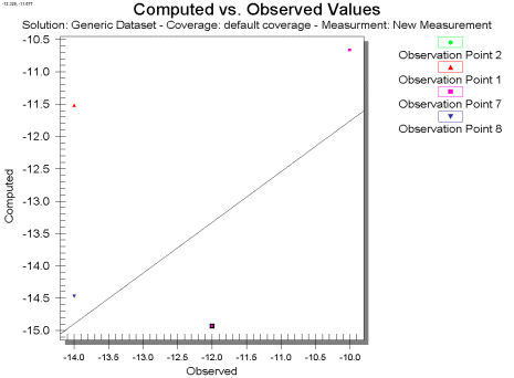
A Computed vs. Observed plot is used to display how well the entire set of observed values for observation points matches the solution data. On this plot is drawn a 45° line, representing what would be a perfect correspondence between observed data and solution values. Then, one symbol is drawn for each observation point at the intersection of the observed and computed values for the point. This plot can show the trend of the solution values with regards to matching the observed data. Only those points whose value is specified as observed for the selected data type will be shown in the plot. These plots are created in the Plot Wizard by setting the Plot Type to Computed vs. Observed Data. A sample plot is shown in the figure below.
Computed vs. Observed Plot Options
After the plot type is set in Step 1 of the Plot Wizard, the Next button is clicked to go to Step 2, which displays the following items.
- Coverage – Displays the name of the coverage where the current data for the plot is coming from.
- Measurement – This is the name of the current measurement, created in the Feature Objects | Attributes dialog, being plotted.
- Feature Objects – Displays which feature object is utilized in the current plot, points or arcs.
- Use current solution – This option causes the plot to compare the observed values with the values of the current solution and time step for each observation point. When the active solution changes, the plot is recomputed and updated. If only one solution is in memory then this option is defaulted.
- Use selected solutions – This option causes the plot to compare the observed values with the values of the specified solution for each observation point. Changing the active solution does not affect the plot.
Computed vs. Observed Troubleshooting
If a plot will not generate or does not display significant data, it's possible that the conditions for the plot have not been set up correctly. To get a meaningful plot, take the following into account:
- This plot requires an observation coverage with feature points included that have observation data from the field.
- This plot requires a simulation with calculated data of the same type of data as the observation coverage (velocity, for example). If the simulation does not have solution datasets, then this plot will not have significant results.
- The dataset desired for visualization should be selected in the Project Explorer. Which dataset is selected affects what displays in the plot.
Related Topics
| [hide] SMS – Surface-water Modeling System | ||
|---|---|---|
| Modules: | 1D Grid • Cartesian Grid • Curvilinear Grid • GIS • Map • Mesh • Particle • Quadtree • Raster • Scatter • UGrid |  |
| General Models: | 3D Structure • FVCOM • Generic • PTM | |
| Coastal Models: | ADCIRC • BOUSS-2D • CGWAVE • CMS-Flow • CMS-Wave • GenCade • STWAVE • WAM | |
| Riverine/Estuarine Models: | AdH • HEC-RAS • HYDRO AS-2D • RMA2 • RMA4 • SRH-2D • TUFLOW • TUFLOW FV | |
| Aquaveo • SMS Tutorials • SMS Workflows | ||
