SMS:BOUSS-2D Using the Model
BOUSS-2D Grid
When using the model, the project will need a BOUSS-2D Cartesian grid. If a grid has already been created or an existing simulation read, the grid object will exist in the Project Explorer and selecting that object will make the Cartesian grid module active.
To create a BOUSS-2D grid:
- Right-click on the Map Data
 item and select New Coverage.
 - Select BOUSS-2D.
- Give the coverage a name then click Ok.
- Click out a grid frame using the Grid Frame tool.
- Follow the instructions found at Creating 2D Cartesian Grids.
Boundary Condition data
All numeric models require boundary condition data. In BOUSS-2D, boundary conditions are defined along arcs for porosity/damping, and on nodes for wave makers.
Damping / Porosity coverage
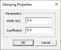
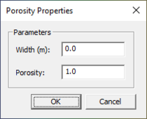
Damping and porosity coverages contain arcs that represent damping/porosity. The location of the arcs will be the location of the damping/porosity when running a simulation. Assigned to the arcs is the attributes of width and value. Multiple arcs can be created in a single coverage.
To create a damping/ porosity coverage:
- Right-click on the Map Data
 item and select New Coverage.
 - Select BOUSS-2D Damping or Porosity.
- Give the coverage a name then click Ok.
- Select the newly created coverage.
- Click on the Create Feature Arc tool.
- Click out an arc over the grid where wanting the damping/porosity.
- Click on the Select Feature Arc tool.
- Click on an arc, then right-click and select Attributes.
Wave Maker Coverage
Wave maker coverages contain points that represent a wave maker. The location of the point will be the location of the wave maker when running a simulation. Assigned to the points are the wave maker settings including type and direction.
To create a wave maker coverage:
- Right-click on the Map Data
 item and select New Coverage.
 - Select BOUSS-2D wave maker.
- Give the coverage a name then click Ok.
- Select the newly created coverage.
- Click on the Create Feature Point tool.
- Click out a point over the grid where wanting the wave maker.
- Click on the Select Feature Point tool.
- Click on an point, then right-click and select Attributes.
Creating a Constant Depth Wave Maker Platform
The BOUSS-2D model generates waves along the specified wave makers (as described above). In order to increase model stability, and allow using an internal wave maker, it is necessary that the depths in the grid under a wave maker be relatively constant. For this reason, wave makers should be positioned far enough off shore that an entire row/column of the grid is at a relatively constant water depth. If the depth varies more than 10%, SMS will issue a warning when outputting the model.
To correct this situation, the depth under the wave maker can be adjusted to a constant value, creating a flat area. (This meets the requirements for stability for the BOUSS-2D model. We refer to this flat area as the wave platform.) The steps to create a flat area include:
- select the cells of the area to be made flat (directly under and adjacent to the wave maker). Use the select cell, select row or select column tools to do this.
- specify the elevation (remember that BOUSS-2D uses elevations, so depths are negative numbers) in the Z edit field to change the elevation of the selected area.
Example
- Assume the grid origin (I=1, J=1)is offshore, and wanting to place the wave maker at the I=50 column.
- Assume the average elevation of all cells between I=1 and I=50 is -30 m.
Steps
- Select all the cells in columns 1 through 50
- Specify an elevation of -30 m in the Z edit field
Notes
- SMS computes the average depth of all selected cells. This is displayed in the Z edit field when multiple cells are selected.
- The average depth could be chosen by selecting the row or column where the wave maker will be placed. However,
- Selecting a few rows/columns using the shift key to add to the selection in the region of the wave maker displays the average elevation for a larger region. This average may blend into the natural bathymetry with less the irregularity.
- Individual rows/columns can be selected with the SMS grid tools. Larger regions can be selected using the select cell tool and holding down the control key and dragging a box. The alt key can be used to just add new cells to the selection list.
- The constant elevation area should extend for several columns/rows behind and in front of the wave maker. The rule of thumb is to select all the rows/columns within half-wavelength from the wave maker.
Creating a Transition Zone from Wave Maker Platform to Natural Bathymetry
If a constant elevation area has been created as described in the previous section, rapid changes in elevations past the wave maker can cause model instabilities. To avoid this, it is recommended to create a smoothed transition zone shoreward of the wave maker by smoothing the bathymetry. Otherwise, the BOUSS-2D model may still encounter instabilities do to rapid changes in bathymetry. To avoid this potential problems, use SMS to smooth the bathymetry to transition smoothly from the wave maker into the natural bathymetry. (Note: this operation should only be applied in area close to the wave maker, and no smoothing should be made to the principal study area. The effect of bathymetry smoothing on model results depends on the magnitude and extent of smoothing applied.
To create a smooth transition, use the following steps:
- Right-click on the grid and convert the grid to a scatter set.
- Switch to the scatter module and make sure the newly created scatter set is active.
- Issue the Data | Dataset Toolbox... command to bring up the toolbox.
- Select the Smooth datasets command.
- Select the dataset which represents the bathymetry values.
- Select the option to limit the Maximum slope and enter the transition value. (i.e. 0.1 implies a maximum slope of 1 on 10)
- Select the option to anchoe the Minimum value. This assumes that the wave platform is the minimum value and will ensure that it stays flat as defined in the section above.
- Enter a new dataset name such as ramped_bathy to store the smoothed bathymetry dataset.
- Click the Compute button to generate the new dataset and then the Done button to exit the toolbox.
- Switch back to the grid module and select the Select Cell tool.
- Drag a box (control key) around the wave platform and the adjacent area where the grid transition is to be applied. This will select the cells that will represent this transition.
- Right-click on any of the selected cells and select the Interpolate Bathymetry... command.
- Select the ramp_bathy function (using the name used in the step above) to select the new bathymetry source for the selected cells and click the OK button.
Note: The above steps replace the natural bathymetry in the grid only in the transition zone. If wanting to save this, duplicate the dataset before applying this smoothing operation. Also note that the bathymetry smoothing of the dataset is applied to the entire region. The coastline and any structures along the coastline would also be smoothed. That is why the application of the new bathymetry is limited to the selected cells in the vicinity of wave maker in the final steps of this procedure.
Using Roughness Coefficients
Roughness coefficients can be defined in a roughness coverage then converted to the active grid.
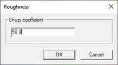
The BOUSS-2D roughness coverage allows building polygons that can be assigned a roughness coefficient. Right-click on a feature polygon and selecting the Attributes command with bring up a Roughness dialog.
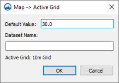
After setting the roughness coefficient for the polygons, the roughness coverage can be converted to the active grid. The grid that is currently selected in the Project Explorer will receive the roughness dataset. Right-clicking on the roughness coverage in the Project Explorer and selecting the Convert | Map → Active Grid will bring up the Map → Active Grid dialog. The Map → Active Grid dialog allows setting a default roughness coefficient value and assigning a dataset name for the roughness coefficient dataset being assigned to the active grid.
Related Topics
SMS – Surface-water Modeling System | ||
|---|---|---|
| Modules: | 1D Grid • Cartesian Grid • Curvilinear Grid • GIS • Map • Mesh • Particle • Quadtree • Raster • Scatter • UGrid |  |
| General Models: | 3D Structure • FVCOM • Generic • PTM | |
| Coastal Models: | ADCIRC • BOUSS-2D • CGWAVE • CMS-Flow • CMS-Wave • GenCade • STWAVE • WAM | |
| Riverine/Estuarine Models: | AdH • HEC-RAS • HYDRO AS-2D • RMA2 • RMA4 • SRH-2D • TUFLOW • TUFLOW FV | |
| Aquaveo • SMS Tutorials • SMS Workflows | ||


