GMS:Natural Neighbor
The basic equation used in natural neighbor interpolation is identical to the one used in IDW interpolation:
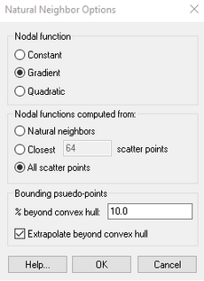
As with IDW interpolation, the nodal functions can be either constants, gradient planes, or quadratics. The nodal function can be selected using the Natural Neighbor Interpolation Options dialog. The difference between IDW interpolation and natural neighbor interpolation is the method used to compute the weights and the method used to select the subset of point data used for interpolation.
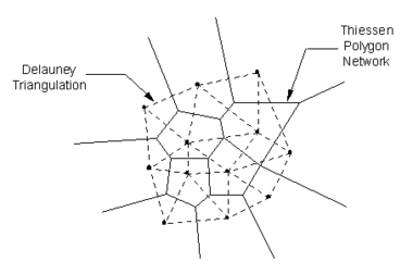
Natural neighbor interpolation is based on the Thiessen polygon network of the point data. The Thiessen polygon network can be constructed from the Delaunay triangulation of a set of points. A Delaunay triangulation is a network of triangles that has been constructed so that the Delaunay criterion has been satisfied.
There is one Thiessen polygon in the network for each point. The polygon encloses the area that is closer to the enclosed point than any other point. The polygons in the interior of the points are closed polygons and the polygons on the convex hull of the points are open polygons.
Each Thiessen polygon is constructed using the circumcircles of the triangles resulting from a Delaunay triangulation of the points. The vertices of the Thiessen polygons correspond to the centroids of the circumcircles of the triangles.
Local Coordinates
The weights used in natural neighbor interpolation are based on the concept of local coordinates. Local coordinates define the "neighborliness" or amount of influence any point will have on the computed value at the interpolation location. This neighborliness is entirely dependent on the area of influence of the Thiessen polygons of the surrounding points.
To define the local coordinates for the interpolation location, Pn, the area of all Thiessen polygons in the network must be known. Temporarily inserting Pn into the network of triangles causes the corresponding Thiessen network to change, resulting in new Thiessen areas for the polygons in the neighborhood of Pn.
The concept of local coordinates is shown graphically in the following figure. Points 1-10 are data points and Pn is an interpolation location where some value associated with points 1-10 is to be interpolated. The dashed lines show the edges of the Thiessen network before Pn is temporarily inserted into triangle network and the solid lines show the edges of the Thiessen network after Pn is inserted.
Only those points whose Thiessen polygons have been altered by the temporary insertion of Pn are included in the subset of points used to interpolate a value at Pn. In this case, only points 1, 4, 5, 6, & 9 are used. The local coordinate for each of these points with respect to Pn is defined as the area shared by the Thiessen polygon defined by point Pn and the Thiessen polygon defined by each point before point Pn is added. The greater the common area, the larger the resulting local coordinate, and the larger the influence or weight the point has on the interpolated value at Pn.
If the user defines k(n) as the Thiessen polygon area of Pn and km(n) as the difference in the Thiessen polygon area of a neighboring scatter point, Pm, before and after Pn is inserted, then the local coordinate lm(n) is defined as:
The local coordinate lm(n) varies between zero and unity and is directly used as the weight, wm(n), in the interpolation equation. If Pn is at precisely the same location as Pm, then the Thiessen polygon areas for Pn and Pm are identical and lm(n) has a value of unity. In general, the greater the relative distance Pm is from Pn, the smaller its influence on the final interpolated value.
Extrapolation
As shown in the figure above, the Thiessen polygons for data points on the perimeter of the triangle network are open-ended polygons. Since such polygons have an infinite area, they cannot be used directly for natural neighbor interpolation. Thus, a special approach is used to facilitate extrapolation with the natural neighbor scheme. Prior to interpolation, the X and Y boundaries of the object being interpolated to (grid, mesh, etc.) are determined and a box is placed around the object whose boundaries exceed the limits of the object by approximately 10% (this value can be modified). Four temporary "pseudo points" are created at the four corners of the box. The inverse distance weighted interpolation scheme with gradient plane nodal functions is then used to estimate a data value at the pseudo-points. From that point on, the pseudo-points with the extrapolated values are included with the actual data points in the interpolation process. Consequently, all of the points being interpolated to are guaranteed to be within the convex hull of the data points. Once the interpolation is complete, the pseudo-points are discarded.
See also
GMS – Groundwater Modeling System | ||
|---|---|---|
| Modules: | 2D Grid • 2D Mesh • 2D Scatter Point • 3D Grid • 3D Mesh • 3D Scatter Point • Boreholes • GIS • Map • Solid • TINs • UGrids | |
| Models: | FEFLOW • FEMWATER • HydroGeoSphere • MODAEM • MODFLOW • MODPATH • mod-PATH3DU • MT3DMS • MT3D-USGS • PEST • PHT3D • RT3D • SEAM3D • SEAWAT • SEEP2D • T-PROGS • ZONEBUDGET | |
| Aquaveo | ||


