SMS:CMS-Flow Model Control
The CMS-Flow Model Control dialog allows viewing and editing the current parameters that affect how CMS-Flow runs and what options are to be included in the current simulation. The Model Control dialog is access by right-clicking on the CMS-Flow simulation object and selecting the Model Control command.
The dialog includes several tabs which partition the parameters into related groups. The tabs and their related parameters include:
General
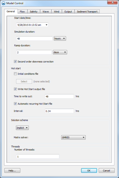
Specifies general flow model parameters, controlling which model options the simulation will employ. The controls include:
Time Control
This section sets the starting time, duration and hydraulic time step. The Ramp duration defines the length of an incremental loading portion at the beginning of the simulation. Controls include:
- Start date/time – The hour and day at which to begin the model. This will be the first time step listed in any solution files.
- Simulation duration – the length of the simulation in hours.
- Ramp duration – The period of time in days at which to allow the model to “build up” or “ramp up” to a legitimate solution. Aids in the convergence of the model.
- Second order skewness correction – Turns on or off the second order skewness correction which account for non-orthogonality in the telescoping grids.
Hot Start
These controls allow specifying a previously saved hot start file to be used as initial conditions or instruct CMS-Flow to save hot start files for future use.
- Initial conditions file
- Write Hot Start output file
- Time to write out
- Automatic recurring Hot Start file
- Interval for writing recurring Hot Start file
See CMS-Flow Hot Start File for more information.
Solution Scheme
CMS-Flow now has two solution schemes. These include the traditional "explicit" scheme. This method requires that flow be tracked through each element, resulting in hydrodynamic time steps in the order of one to two seconds. The new option is an "implicit" scheme which uses finite volume technology, supports much larger time steps resulting in fewer time steps (shorter run times) and is identically mass conserving. When the implicit scheme is being used, one of the following matrix solver types should be specified.
- Solution scheme – Can be set as "Implicit" or "Explicit".
- Matric solver – Can be specified when using the "Implicit" option. Options are "Gauss-Seidel", "Gauss-Seidel-SOR", "BiCGSTab", or "GMRES".
Threads
CMS-Flow can take advantage of multiple processors using Open-MP parallelization technology. This control allows specifying the maximum number of threads that the engine should occupy.
- Number of threads – Determines the number of threads used for parallel processing.
Flow
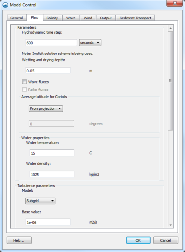
Specifies general hydrodynamic or flow model parameters, controlling which model options the simulation will employ. The controls include:
Hydrodynamic Time Step
This control allows setting the hydrodynamic time step for the model. If the explicit solution scheme is being used, a recommended time step will be calculated based on grid cell size and depths.
- Hydrodynamic time step – Sets the time step for the hydrodynamics.
- Wetting and drying depth – Sets the minimum depth for wet cells.
- Wave fluxes – Turns on and off the wave volume flux velocities.
- Roller fluxes – Turns on or off the contribution to the wave volume flux velocities due to the surface roller in the surf zone. Only used if surface roller model is turned on.
- Average latitude for Coriolis – Specifies the average latitude for the grid which is used for the Coriolis parameter.
Water Parameters
This section allows specifies various general parameters to be used by the simulation. This include:
- Water temperature – Used in the calculation of the water kinematic viscosity and water density if not specified.
- Water density – Assumed to be constant for the simulation. If not specified, calculated based on the water temperature and salinity.
Turbulence Parameters
Specifies turbulence parameters.
- Model – Specifies the turbulence model used: "Subgrid", "Falconer", "Parabolic", or "Mixing length".
- Base value – Constant contribution of eddy viscosity.
- Current bottom coefficient – Coefficient related to the contribution to eddy viscosity from the bottom shear.
- Current horizontal coefficient– Coefficient related to the contribution to eddy viscosity from horizontal velocity gradients.
- Wave bottom coefficient – Coefficient related to the wave bottom friction contribution to eddy viscosity.
- Wave breaking coefficient – Coefficient related to the wave breaking contribution to eddy viscosity.
Bottom and Wall Friction
Friction datasets can be created and specified to define a spatially variable bottom roughness to provide a resistance to flow. This value has little impact in deep ocean applications but can be important in shallow regions. This is a user editable dataset. The available dataset types are:
- Wave-current bottom friction coefficient – Used for quadratic com-bined wave-current mean bed shear stress calculation.
- Coefficient
- Bed-slope friction coefficient – Specifies whether to include the bed slope friction factor or not in the calculation of the bed friction.
- Wall friction – Turns on or off wall friction.
- Bottom roughness dataset
Salinity
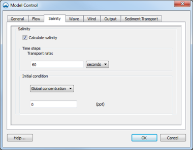
Specifies model parameters relating to salinity modeling in CMS-Flow. The controls include:
- Calculate salinity – Turning on this option allows specifying the salinity options. If this is option is not used, salinity will not be included in the model run.
Time Steps
In addition to the time step specified in the general parameters tab for hydrodynamic calculations, the explicit model also allows the specification of longer time step for the salinity dispersion process.
- Transport rate – Specify this time step if salinity is enabled in this tab and the solver option is set to "explicit" in the Flow tab. It must be larger than the hydrodynamic time step and is generally at least a factor of 20. The default transport rate time step is 60 seconds.
Initial Condition
Salinity transport requires that each cell have an initial value for salinity concentration (measured in ppt). CMS-Flow allows this value to start as a constant for each cell, in which case, during the initial (or ramp time)of the simulation the concentrations are distributing to natural values.
- "Global concentration" – This control specifies an initial concentration for the entire domain. The value 0.0 ppt (fresh water) is a commonly used value.
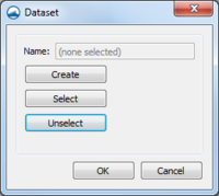
- "Spatially varied" – This option allows to bring up a Dataset dialog where it is possible to create or select a spatially varied dataset that will be used by CMS-Flow as the initial concentration at each cell. The Dataset dialog has the following options:
- Create – Brings up the Dataset Toolbox where a new dataset can be created using the Data Calculator.
- Select – Brings up an option to select an existing dataset already in the project.
- Unselect – Removes the selected or created dataset.
Wave Data
CMS-Flow includes three options on how to use wave data.
None
No wave data is imputed into the model.
Single wave condition
The effects of waves are input to the model in the form of spatially varying datasets. These datasets must already exist on the grid. Simply select which dataset to use.
- Significant wave height
- Peak wave period
- Mean wave direction
- Wave breaking dissipation
- Wave radiation stress gradients
- Surface roller stress gradients
Clicking on the Select button under any of the options with being up a Dataset dialog with two options. The Select button in the Dataset dialog will bring up a Select Dataset dialog where a dataset in the project can be chosen. The Unselect button will remove the selected dataset.
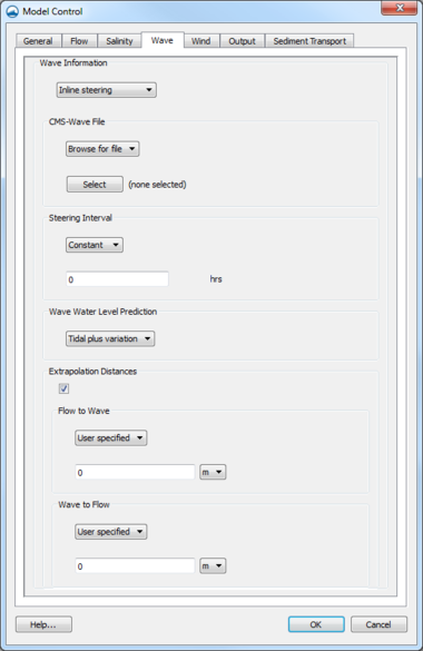
Inline steering
- CMS-Wave file – Location of the grid file or the simulation file. Can either "Browse for file" or use the "Wave grid".
- Steering Interval – Sets the recurring hot start output time. Option to use a "Constant" value or "Automatic" value.
- Wave Water Level – Determines the method used to calculate the water levels passed to the wave model. Option to select "Tidal", "Last time step", or "Tidal plus variation" (default value).
- Extrapolation Distances – If checked this will write out FLOW_EXTRAPOLATION_DISTANCE and WAVE_EXTRAPOLATION_DISTANCE cards.
- Flow to Wave – Determines the extrapolation distance used for flow variables on the wave grid. Option to set a "User specified" value or "Automatic" value.
- Wave to Flow – Determines the extrapolation distance used for wave variables on the flow grid. Option to set a "User specified" value or "Automatic" value.
Wind Data
Turn on the option to tell CMS to include wind calculations in the simulation. Wind is simulated in CMS-Flow as a spatially constant, but temporally varying quantity. The model does not currently support tropical cyclonic winds.
For more wind file information, see: CMS-Flow Wind Forcing on the CIRP wiki.
None
No wind data is imputed into the model.
Spatially constant
- Parameters – Set through the time series editor below. Clicking the
 button will add a row to the editor and clicking the
  button will remove a row. The follow options can be specified in each row:
- Time (hr) – Specify time of wind measurement.
- Direction (deg) – Specify the variation in direction of the wind in the simulation.
- Velocity (m/s) – Specify the variation of wind velocity in the simulation.
- Anemometer height (m)
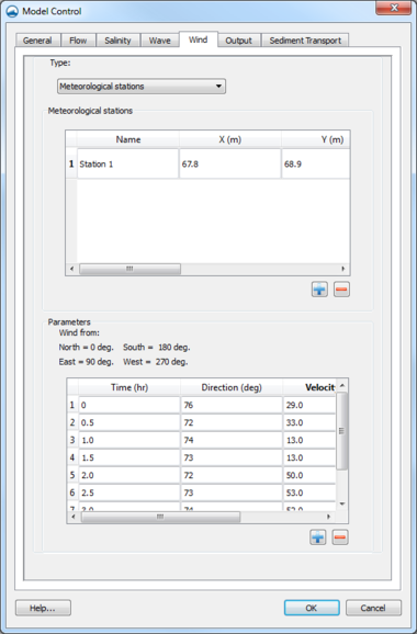
Meteororological stations
This option allows inserting data for multiple locations
- Mereorological stations – This section contains a properties editor where each station can be defined. A station is added using the
 button or removed using the
  button. The options are:
- Name – The designated name of the station.
- X(m) – X-axis location of meteorologic station.
- Y(m) – Y-axis location of meteorologic station.
- Height (m)
- Direction Curve – Launches an XY Series Editor window.
- Parameters – Set through the time series editor below. Clicking the
 button will add a row to the editor and clicking the
  button will remove a row. The follow options can be specified in each row:
- Time (hr) – Specify time of wind measurement.
- Direction (deg) – Specify the variation in direction of the wind in the simulation.
- Velocity (m/s) – Specify the variation of wind velocity in the simulation.
Temporally and spatially varying from file
The File Type chosen will determine the rest of the options available for wind type. There are three File Type options available:
- "Navy fleet numeric with pressure "
- "OWI/PBL"
- "Single ASCII file"
Navy fleet and ASCII files require the following input under "Parameters":
- Number of values (X)
- Number of values (Y)
- Minimum X location
- Maximum Y location
- Time increment(s)
- Distance between X values (m)
- Distance between Y values (m)
Alternatively, the "XY File" option can be selected and a file imported with the above parameters.
OWI/PBL requires three different files:
- Oceanweather Wind File
- Oceanweather Pressure File
- Oceanweather XY File
Output
This dialog allows specifying global output options for the simulation. This controls the datasets created by the engine which consist of spatially and temporally varied quantities (values per cell at each output time value).
These output datasets are stored in their respective XMDF (*.h5) files (e.g. current velocity in vel.h5 and water surface elevation in wse.h5). In previous versions of CMS-Flow all the datasets were stored in a single solution (sol.h5) file, though that is not an option in current versions.
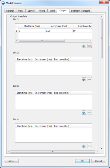
Output Times Lists
Due to the potentially long simulation times, CMS-Flow does not output at a constant interval during the simulation. Instead, define one or more lists of times. Select one time list for each dataset output by the engine. The selected quantity will be saved at each time in the time list.
CMS-Flow supports up to four different and individual sets of time values. The options for each list include:
- Start time (hrs)
- Increment (hrs)
- End time (hrs)
Each list can have multiple time sets. To add a time set, click on the Add (+) button. To remove a time set, click on the Remove (-) button.
Output Datasets
CMS-Flow can output each of the following datasets. For each group, a time list must be specified. The optional datasets may turned off/on by clicking on their checkboxes in the output dataset tree.
- Water Surface Elevation
- Current Velocity
- Current Magnitude (optional)
- Current Velocity
- Morphology
- Depth (through time)
- Morphology Change (optional)
- Transport
- Sediment Total-Load Capacity (optional)
- Sediment Total-Load Concentration (optional)
- Fraction Suspended (optional)
- Total Sediment Transport
- Salinity Concentration (optional)
- Waves
- Wave Height
- Wave Period
- Wave Height Vector
- Wave Dissipation (optional)
- Wind
- Wind Speed (optional)
- Wind Speed Vector
- Eddy Viscosity
Statistical Output
Statistical data can be written out for the following:
- Hydrodynamics
- Sediment Transport
- Salinity
The options are turned on by toggles. For any option that is turn on, specify the following:
- Start time (hrs)
- Increment (hrs)
- End time (hrs)
Output Options
Output can be written out in ASCII format and the XMDF files can be compressed. These options are turned on by toggle boxes. All datasets created by the model will be labeled with a simulation label and quantity label.
The following file output options are available:
- Tecplot snap shot (*.dat) and history files (*.his)
- SMS Super ASCII files (*.sup, *.xy, *.dat)
- XMDF file compression
- Simulation label – Specify a name for output files.
Sediment Transport
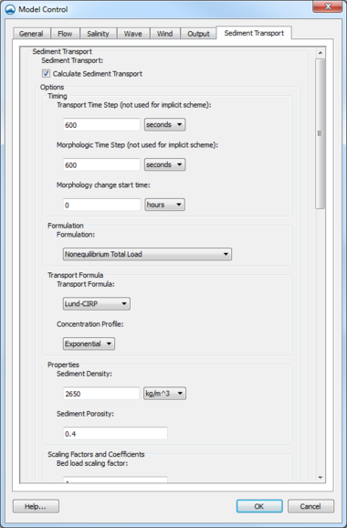
Sediment transport options can be specified by toggling on the Calculate Sediment Transport option in the Model Control. Once this option is selected, sediment transport data will be calculated during the model run.
More information on sediment transport can be found at: Two-Dimensional Depth-Averaged Circulation Model CMS-M2D: Version 3.0, Report 2, Sediment Transport and Morphology Change[1]
The options for sediment transport are:
Timing
The sediment transport and morphologic time steps are the time steps at which the transport and bed change equations are calculated.
- Transport Time Step (not used for implicit scheme) – Used for transport equation.
- Morphologic Time Step (not used for implicit scheme) – Used for updating bed elevation.
- Morphologic change start time – Sets start time for the morphology change calculation.
Formulation
- "Equilibrium Total Load" – Assumes both the bed load and suspended load to be in equilibrium. The bed change is solved using a simple mass balance equation known as the Exner equation.
- "Equilibrium Bed load plus Nonequilibrium Susp Load" – Conducted separately the calculations of suspended load and bed load. The bed load is assumed to be in equilibrium and is included in the bed change equation while the suspended load is solved through the solution of an advection-diffusion equation. Actually the advection diffusion equation is a non-equilibrium formulation, but because the bed load is assumed to be in equilibrium, this model is referred to the "Equilibrium A-D" model.
- "Nonequilibrium Total Load" – Assumes neither the bed nor suspended loads to be in equilibrium. The suspended- and bed-load transport equations are combined into a single equation and thus there is one less empirical parameter to estimate (adaptation length).
Transport Formula
- Transport Formula – Selects the transport formula.
- "Lund-CIRP"
- "van Rijn"
- "Soulsby-van Rijn"
- "Watanabe"
- Concentration Profile – Selects the concentration profile to be used either in the equilibrium A-D or NET models. In the A-D model, it is used to estimate the near bed concentration, whereas in the NET, it is used in the total load correction factor.
- "Exponential"
- "Rouse"
- "Lund-CIRP"
- "van Rijn"
- Watanabe Transbort Rate Coefficient – Sets the empirical coefficient which goes into the Watanabe transport formula.
Properties
- Sediment Density – Sets the sediment density in kg/m^3.
- Sediment Porosity – Sets the sediment porosity.
Scaling Factors and Coefficients
- Bed load scaling factor – Calibration factor for bed load transport capacity formula
- Suspended load scaling factor – Calibration factor for suspended load transport capacity formula
- Morphologic acceleration factor – Directly multiplies by calculated bed change.
- Bed slope diffusion coefficient
- Hiding and exposure coefficient
Adaptation
The adaptation coefficient is an important parameter to consider in setting up the CMS sediment transport model. The sensitivity of results to the adaptation coefficient depends on the spatial and temporal scales of the problem.
- Total load adaptation method
- "Constant length" – Temporally and spatially total load adaptation length is used for the whole domain.
- Total load adaptation length
- "Constant time" – Temporally and spatially constant total-load adaptation time is used for the whole domain.
- Total load adaptation time
- "Maximum of bed and suspended adaptation lengths" – Temporally and spatially constant total-load adaptation time that uses a maximum suspended load adaptation length and maximum bed load adaptation length.
- Bed load adaptation method – Specifies the bed load adaptation coefficient method. Options include:
- "Constant Length" – Allows specifying a Bed load adaptation length.
- "Constant Time" – Specifies the bed-load adaptation time.
- "Depth Dependent" – Allows specifying a Bed load adaptation depth factor.
- Suspended load adaptation method – Specifies the suspended load adaptation coefficient method. Options include:
- "Constant length" – Allows specifying a Suspended adaptation length.
- "Constant time" – Allows specifying a Suspended adaptation time.
- "Constant coefficient" – Allows specifying a Suspended adaptation coefficient.
- "Armanini and Di Silvio"
- "Lin"
- "Gallappatti"
- "Weighted average of bed and suspended adaptation lengths" – Has options similar to the "Maximum of bed and suspended adaptation lengths" option. A temporally and spatially constant total-load adaptation time that uses a suspended load adaptation length, a bed load adaptation length, and a fraction of suspended load of the total load.
Size Classes
The transported sediment material is discretized into different groups each representing the sediments within a specific size range.
- Sediment size class diameters – To add a sediment class, click on the
 button. To remove a sediment class, click on the
  button.
- Diameter – Sediment size class characteristic diameter.
- Fall Velocity Method – Sediment size class fall velocity formula.
- Fall Velocity – Sediment size class fall velocity.
- Cory Shape Factor – Sediment size class Corey Shape Factor. Used in the Wu and Wang (2006) sediment fall velocity formula.
- Critical Sheer Method – Sediment size class characteristic critical shear stress formula.
- Critical Sheer Stress (Pa) – Sediment size class characteristic critical shear stress.
Bed Composition
The initial bed layer thickness and composition are specified at least one layer for the whole grid.
- Bed layer block – To add a bed layer block, click on the
 button. To remove a bed layer block, click on the
  button.
- Layer ID – Specifies the bed layer number from the surface. If not specified then set the sequential bed layer block number.
- Thickness Dataset – Specifies the file name and dataset path (within the file) for the bed layer thickness dataset.
Percentile Diameters – Indicate the percentage of diameters smaller than a specific diameter.
- D05
- D10
- D16
- D20
- D30
- D35
- D50
- D65
- D84
- D90
- D95
Avalanching
Avalanching is the process of sediment sliding when the critical angle of repose is reached.
- Calculate Avalanching – Turns on or off the avalanching.
- Critical bed slope – Specifies the sediment repose angle. Avalanching is activated when the bed slope exceeds the repose angle.
- Maximum number of iterations (implicit only) – Maximum number of iterations for implicit solution scheme. When using the explicit scheme, one iteration is performed every time step.
Hardbottom
A morphologic constraint that provides the capability to simulate mixed bottom types within a single simulation.
- Hardbottom depth – Turning on this option and using the Select button will bring up a Dataset dialog. The Dataset dialog has the following options:
- Create – Brings up the Dataset Toolbox where a new dataset can be created using the Data Calculator.
- Select – Brings up an option to select an existing dataset already in the project.
- Unselect – Removes the selected or created dataset.
Related Topics
| [hide] SMS – Surface-water Modeling System | ||
|---|---|---|
| Modules: | 1D Grid • Cartesian Grid • Curvilinear Grid • GIS • Map • Mesh • Particle • Quadtree • Raster • Scatter • UGrid |  |
| General Models: | 3D Structure • FVCOM • Generic • PTM | |
| Coastal Models: | ADCIRC • BOUSS-2D • CGWAVE • CMS-Flow • CMS-Wave • GenCade • STWAVE • WAM | |
| Riverine/Estuarine Models: | AdH • HEC-RAS • HYDRO AS-2D • RMA2 • RMA4 • SRH-2D • TUFLOW • TUFLOW FV | |
| Aquaveo • SMS Tutorials • SMS Workflows | ||
