SMS:Computed vs. Observed Data Plot
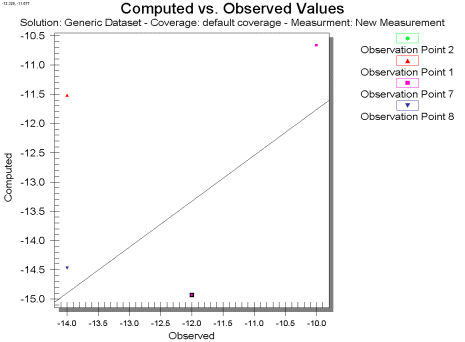
A Computed vs. Observed plot is used to display how well the entire set of observed values for observation points matches the solution data. On this plot is drawn a 45° line, representing what would be a perfect correspondence between observed data and solution values. Then, one symbol is drawn for each observation point at the intersection of the observed and computed values for the point. This plot can show the trend of the solution values with regards to matching the observed data. Only those points whose value is specified as observed for the selected data type will be shown in the plot. These plots are created in the Plot Wizard by setting the plot type to Computed vs. Observed. A sample plot is shown in the figure below.
Computed vs. Observed Plot Options
After the plot type is set in Step 1 of the Plot Wizard, the Next button is clicked to go to Step 2, which displays the following items.
- Coverage – Displays the name of the coverage where the current data for the plot is coming from.
- Measurement – This is the name of the current measurement, created in the Feature Objects | Attributes dialog, being plotted.
- Feature Objects – Displays which feature object is utilized in the current plot, points or arcs.
Related Topics
SMS – Surface-water Modeling System | ||
|---|---|---|
| Modules: | 1D Grid • Cartesian Grid • Curvilinear Grid • GIS • Map • Mesh • Particle • Quadtree • Raster • Scatter • UGrid |  |
| General Models: | 3D Structure • FVCOM • Generic • PTM | |
| Coastal Models: | ADCIRC • BOUSS-2D • CGWAVE • CMS-Flow • CMS-Wave • GenCade • STWAVE • WAM | |
| Riverine/Estuarine Models: | AdH • HEC-RAS • HYDRO AS-2D • RMA2 • RMA4 • SRH-2D • TUFLOW • TUFLOW FV | |
| Aquaveo • SMS Tutorials • SMS Workflows | ||
