GMS:Variogram Editor
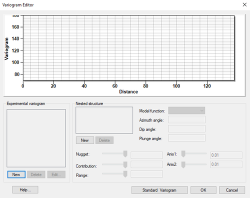
Before interpolating a scatter point set using the Kriging option, a model variogram must be defined. The basic steps involved in constructing a model variogram are to first build an experimental variogram and then construct a model variogram that matches the experimental variogram. This is accomplished using the Variogram Editor. The Variogram Editor is activated by selecting the Edit Variogram button in the Kriging Options dialog.
The experimental variograms and the model variogram are plotted in the upper portion of the Variogram Editor. The items in the upper right portion of the editor are used to create experimental variograms. The items in the lower half of the editor are used to define the model variogram. In a typical study, several experimental variograms may be constructed and plotted before one is chosen. A model variogram is then designed to fit the chosen experimental variogram.
Creating Experimental Variograms
A new experimental variogram is computed by selecting the New button under the list of experimental variograms. This button brings up the Experimental Variogram dialog.
Lags
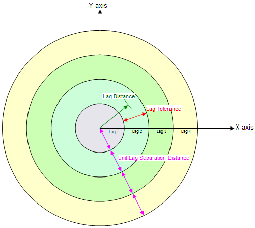
When computing an experimental variogram, it is impractical to plot a variance for each scatter point with respect to each of the other scatter points. Therefore, distances are subdivided into a number of intervals called lags as illustrated in the following figure. The distance between each pair of scatter points is checked to see which lag interval it lies within. The variances for all pairs of points whose separation distance falls within the same lag interval are averaged. The resulting average is plotted in the experimental variogram vs. the distance corresponding to the lag interval. Therefore, there is one point in the experimental variogram plot for each lag. The lag intervals are defined in the Experimental Variogram dialog by entering a total number of lags, a unit lag separation distance, and a lag tolerance. In most cases, the lag tolerance should be one half of the unit lag separation distance; the tolerance can be smaller to allow for data on a pseudo-regular grid. A pair will be included in multiple lags if the tolerance is greater than one-half of the unit lag separation distance.
Semivariogram
The semivariogram is the most common type of variogram. The semivariogram value for a lag interval is computed as:
where N is the number of pairs of points whose separation distance falls within the lag interval and f1i and f2i are the values at the head and tail of each pair of points. The head and tail are defined as follows:
Covariance
The covariance is the traditional covariance used in statistics. The covariance value for a lag interval is computed as:
where m-h and m+h are the mean of the head and tail values respectively.
Correlogram
The correlogram is computed by standardizing the covariance by the standard deviation of the head and tail values.
where s-h and s+h are the standard deviation of the head and tail values respectively.
General Relative Semivariogram
This variogram is computed by standardizing the semivariogram computed using equation 9.38 by the squared mean of the data values in each lag:
Pairwise Relative Semivariogram
With this variogram, each pair is normalized by the squared average of the tail and head values.
Experience has shown that the general relative and pairwise relative semivariograms are effective in revealing spatial structure and anisotropy when the scatter points are sparse (Deutsch & Journel, 1992). Because of the divisors in equations 9.41 and 9.42, these semivariograms should only be used on positively skewed datasets.
Semivariogram of Logarithms
This variogram is computed by applying equation 9.38 to the natural logarithms of the data values:
Semirodogram
The semirodogram is similar to the traditional semivariogram except that the square root of the absolute difference is used rather than the squared difference:
Semimadogram
The semimadogram is similar to the traditional semivariogram, except that the absolute difference is used rather than the squared difference:
The semirodogram and the semimadogram are particularly effective for establishing range and anisotropy. They should not be used for modeling the nugget of semivariograms (Deutsch & Journel, 1992).
Viewing the Experimental Variograms
After setting up the lag interval and choosing a variogram type, the OK button is selected in the Experimental Variogram dialog. At this point, the experimental variogram is computed. For large scatter point sets, this may take a significant amount of time.
Once the experimental variogram is computed, it is added to the list of experimental variograms in the upper right corner of the Variogram Editor and it is displayed in the variogram plotting window. One of the variograms in the list is always highlighted. The name, color, and symbols (used to plot the variogram) of the highlighted variogram can be edited. In addition, the display of each variogram can be turned on and off so any combination of experimental variograms can be plotted. Selecting the Delete button deletes the highlighted variogram. Selecting the Edit button causes the Experimental Variogram dialog to come up initialized with the values used in the computation of the highlighted variogram. When the OK button is selected, the values of the variogram are recomputed.
Creating Model Variograms
Once a set of experimental variograms are computed, one is chosen and a model variogram is constructed to fit the experimental variogram. The model variogram is constructed using the items in the lower half of the Variogram Editor.
Model Functions
Four types of model functions are supported for building model variograms. Each of the functions are characterized by a nugget, contribution, and range.
The nugget represents a minimum variance. The contribution is sometimes called the "sill" and represents the average variance of points at such a distance away from the point in question that there is no correlation between the points. The range represents the distance at which there is no longer a correlation between the points.
The four model functions supported are:
Spherical Model
The Spherical Model is defined by a range -a- and a contribution -c- as:
Exponential Model
The Exponential Model is defined by a parameter -a- and a contribution -c- as:
Gaussian Model
The Gaussian Model defined by a parameter -a- and a contribution -c- as:
Power Model
The Power Model is defined by a power 0 < a < 2 and a slope c as:
Nested Structures
A model variogram is constructed using a combination of one or more model functions. Each instance of a model function is called a "nested structure". A nested structure is created by selecting the New button in the Nested Structure section of the dialog. A new structure is created and added to the list of nested structures. The model variogram plotted in the variogram plot window represents the combination of all of the nested structures in the list. One of the nested structures in the list is highlighted at all times. The selected structure can be deleted by selecting the Delete button under the list. The name, model function type, contribution, and range of the selected structure can be edited (the nugget is the same for all nested structures, i.e., only the contribution and range of each structure are summed). As the parameters defining the structure are altered, the plot of the model variogram is updated dynamically in the variogram plot window. This type of instantaneous feedback provides a powerful tool for "sculpting" a model variogram in an intuitive manner until it fits the selected experimental variogram.
In most cases, a single nested structure is adequate. For cases with complex experimental variograms, using multiple nested structures to define the model variogram can prove useful.
Modeling Anisotropy
Some datasets exhibit anisotropy, i.e., the correlation between scatter points changes with direction. For example, due to the depositional history of an alluvial soil deposit, parameters such as porosity and hydraulic conductivity may be most strongly correlated in one direction. This means the differences in the data values change relatively little in one direction compared to how much they change with distance in the orthogonal direction. The direction corresponding to the highest correlation (smallest change) is called the major principal direction and the orthogonal direction is the minor principal direction.
One of the more powerful features of the kriging method is that anisotropy can be detected by generating experimental variograms in orthogonal directions and looking for differences. When anisotropy exists, the model variogram can be constructed to match the anisotropy and ensure that the differences in the continuity of the data each of the orthogonal directions is accurately modeled in the interpolated dataset.
Detecting Anisotropy
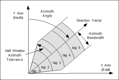
Anisotropy can be detected by generating a focused experimental variogram in each orthogonal direction and observing whether or not there are significant differences in the resulting variograms. When constructing an experimental variogram with the Experimental Variogram dialog, directional data corresponding to an axis of anisotropy can be entered. The meaning of the directional data is illustrated in the following figure:
When a scatter point is compared with each of the other scatter points to compute the experimental variogram, only those points falling within the shaded area shown in the figure above are considered. The shaded area is defined by the azimuth angle, the azimuth bandwidth, the half window azimuth tolerance, and the lag intervals. For isotropic conditions, the half window azimuth tolerance should be set to 90o (the default value). This forces all points to be included in the calculation of the experimental variogram.
Anisotropy is typically detected using a trial and error process. Pairs of experimental variograms are generated, the pairs being offset from each other by an azimuth angle of 90o. If anisotropy exists, the ranges of the two variograms will differ as shown below. If the data are isotropic, the azimuth angle will have little effect on the resulting experimental variograms. The angles which produce the pair of experimental variograms with the largest difference in ranges represent the principal axes of anisotropy. The variogram with the larger range represents the major principal axis and the variogram with the shorter range represents the minor principal axis.
Anisotropy Method
Once anisotropy has been detected, the next step is to model the anisotropy using the model variogram.
The azimuth angle corresponding to that major principal axis (the one with the longer range) should be entered in the azimuth angle field in the lower left corner of the Variogram Editor (the dip and plunge fields are for 3D kriging and are dimmed for 2D interpolation). A model variogram should then be constructed which fits the experimental variogram corresponding to the major principal direction. The anis1 parameter in the Variogram Editor should then be changed to a value other than unity (the default value). Changing the anis1 parameter to a value less than unity causes two curves to be drawn for the model variogram as shown in the above figure. The second curve corresponds to the original curve with the range parameter multiplied by the anis1 value. In other words, the anis1 parameter represents the range in the minor direction divided by the range in the major direction. The anis1 parameter should be altered until the second curve fits the experimental variogram corresponding to the minor principal axis of anisotropy. Each of the nested structures has an anis1 parameter that can be edited. Once again, as the anis1 parameter is altered, the variogram plot is updated dynamically, allowing a fit to be made in a simple intuitive fashion. Once the correct anis1 factor is found, the Variogram Editor should be exited and the azimuth and anis1 factors should be entered in the Search Ellipsoid dialog to define a search ellipse that matches the variogram anisotropy.
Saving Variograms
Once a variogram or set of variograms is defined, the variograms are saved with the dataset files when the project is saved to disk. Thus, when the project is read back in to GMS, the variograms are ready to be used for interpolation and do not need to be redefined.
See also
GMS – Groundwater Modeling System | ||
|---|---|---|
| Modules: | 2D Grid • 2D Mesh • 2D Scatter Point • 3D Grid • 3D Mesh • 3D Scatter Point • Boreholes • GIS • Map • Solid • TINs • UGrids | |
| Models: | FEFLOW • FEMWATER • HydroGeoSphere • MODAEM • MODFLOW • MODPATH • mod-PATH3DU • MT3DMS • MT3D-USGS • PEST • PHT3D • RT3D • SEAM3D • SEAWAT • SEEP2D • T-PROGS • ZONEBUDGET | |
| Aquaveo | ||


