SMS:CGWAVE Practical Notes
Domain Shape: To the extent possible, it is necessary to have the coastlines outside the semicircle be as straight as possible, and ideally, parallel to one of the axis (as shown in Fig 1). The semicircle should be so located that the depths outside vary, to the extent possible, in a 1-d (cross-shore) direction only in the exterior. These depths are introduced in the model through the two 1-d sections. It is necessary to specify a reflection coefficient for the exterior coastline.
Of course, these conditions are not encountered in practice in an ideal manner, but it is important to understand that the model works under these assumptions. V-shaped coastlines do not meet these criteria. Also, not all real domains have 1-dimensionally varying exterior depths. Regions with 2-d depth variations should preferably be incorporated inside the semicircle and it may be necessary to enlarge the domain so that solutions in the area of interest (hopefully) are not affected by the coastline shape. It is impossible to accommodate all real topographic variations of the model’s exterior domain. Since a part of what happens outside the semicircle influences the solution within (i.e. how the backscattered waves behave), some simplified representation of the exterior is needed. The exterior representation used in CGWAVE is more sophisticated than that used in earlier models (which assumed collinear and fully reflecting coastlines and constant exterior depths).
The size of the domain is also governed by the wavelength. Typically, the minimum radius for the semicircle should be about 2 or 3 times the wavelength, which also dictates the overall number of grids. It is important that the modeler first estimate the number of grid points needed, at least in an approximate sense. This can be done by estimating a nominal wavelength L (based on the period and depth), and using L/10 as a rough measure of the grid size. Obviously, large domains with short period waves will lead to hundreds of thousands of nodes. This is not a problem physically, but can be very time consuming to simulate. For spectral conditions, the domain size should be dictated by the longer wavelengths L1 (say radius = 3L1), but the resolution for the shorter wavelengths (L2) would be, say L2/10, which may be excessively fine for the longer wavelengths. Obviously, some care (and perhaps compromise) is needed in designing the grid and also selecting the input spectral components. If some components have little energy, it may be best to delete them from the modeling.
The input wave condition (amplitude, period, direction) must be specified at the end of the 1-d cross-section. Simulations are less reliable (not necessarily wrong) if the waves approach the coast at a glancing angle (say within 20° of the coastline). The 1-d sections MUST reach out further than the outermost point of the semicircle. The domain should have no zero or negative depths; the land-water interface must be demarcated using a small water depth (say 0.5 m, but the limit depends on the overall water depths and wave periods and the problem being solved). Note that making this too shallow may result in a large number of grids in this area which may not be necessary for all applications).
For basic specifications, the incident wave angle specification is as follows. Waves going in the +x axis (i.e. to East) are specified as incident angle =0°. Waves going in +y direction (i.e. to North) are specified as incident angle =90°, to West =180°, to South = 270° . Incident wave direction is used in degrees. Convergence tolerance is typically assigned 10-8, output frequency is 100 every iterations.
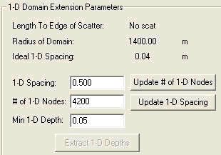
For the boundary condition specification, the “parabolic plus two 1d sections” option (Option 3 in *.cgi) should be chosen for most harbor problems, with a semicircle open boundary; in earlier versions, it is possible to use the option with just one 1d section (Option 2 in *.cgi) but it really provides no benefit over Option 3. The other options consist of the “parabolic approximation” (Option 1 in *.cgi) which is suitable if the exterior region is of constant depth. The Fourier Bessel Series (Option 0 in *.cgi) must be used if its limitations, described above in Section 2.2 (equations 15-17), are met; typically it is sufficient to specify 15 terms in the infinite series. For harbor problems, SMS will create the 1d sections based on depths based on depths on semicircle, and the desired grid spacing (used to solve the 1d equation (20)), based on (approximately) L/10 must be specified in the dialog box:
A full circle option is available for open sea problems where the exterior is of constant depth; the theoretical ideal for this is the Fourier Bessel Series (which works for unit wave input only); the parabolic mode may also be used (Panchang et al. 2000) with little loss of accuracy.
It is useful to perform initial sample runs, with no breaking and with fully absorbing coastlines, for a normally incident and obliquely incident wave input. The resulting solutions, especially the phase diagrams, can be used to perform visual quality control, since forward propagating waves are the easiest for making intuitive assessments (e.g. spacing between crests should be smaller and wave heights generally increasing in shallower water; bending of phase-lines for oblique incidence to approach the shore in a normal fashion, high wave heights in very shallow water because breaking was not applied, etc). Repeating the above runs with full reflection should lead to some standing wave patterns (large and small wave heights; rapid change of phase). A visual examination of the results will enhance confidence in later simulations.
There are two methods for applying wave breaking. For practical problems, we recommend making a non-breaking simulation and then applying an H/d limit (generally between 0.6 and 0.85) to alter the calculated wave heights to the limit (say 0.78d). The other, more rigorous approach is to run the model in the nonlinear breaking mode where breaking properties are continuously recalculated based on prior solutions. This requires several rounds of iterations and is recommended for special problems and/or research applications. For nonlinear runs, the maximum number of nonlinear iterations is generally specified as 15 with a tolerance of 10-6. For spectral simulations, obviously the former approach is recommended.
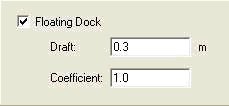
For incorporating docks, the actual “without-dock” water depth is originally specified while generating the grid; areas covering the docks must then be highlighted, and a draft and coefficient, selected from Fig. 2 (Li et al. 2005) or Table 1, must then be specified for these areas. The coefficient = α = Aln(ka)+B. For kh < 0.1 and kh > 4, we recommend using the A and B values corresponding to these thresholds. For convenience, the numerical values corresponding to Figure 8 are given in Table 1. (Note, a = half width of the structure, relative submergence= draft/water-depth = d/h).
For shallow water, α is roughly equal to unity for shallow draft, and α ~ 0.7 for deep draft. For intermediate and deep water, α is not constant but shows an increasing trend with ka. In very deep water, the mismatch is large. Note that for short waves (relative to submergence), T tends to 0. This requires us to create a high level of wave blockage, which can be accomplished by α ~ 0 (Li et al. 2005). Of course this result would not hold if d/h were much smaller than the smallest value investigated by Li et al. (2005), which is 0.25 (typical in engineering practice).
It is worthwhile to refine the grid in these areas since the model uses the under-keel clearance multiplied by the coefficient as the depth for calculation. This modified depth is smaller than the original depth (and hence the resolution should be finer).
Finally, it is noted an extensive list of test-cases are provided in the appendix. CGWAVE has been validated against these tests (which represents possibly the most rigorous testing for wave models). The model results are compared to lab data or analytical model results. The input and output files are provided. It is highly encouraged to perform these simulations, alter parameters, etc. so that an examination of the results may help show what can be expected. At a minimum, we recommend a visual inspection of the results provided. Often real-life problems have complex solutions which are difficult to explain or even anticipate. The fact that the model reproduces the correct result in so many cases may enhance confidence in the results, assuming the modeling was performed with due diligence. The test-cases can also be used as a teaching tool.
Related Topics
| [hide] SMS – Surface-water Modeling System | ||
|---|---|---|
| Modules: | 1D Grid • Cartesian Grid • Curvilinear Grid • GIS • Map • Mesh • Particle • Quadtree • Raster • Scatter • UGrid |  |
| General Models: | 3D Structure • FVCOM • Generic • PTM | |
| Coastal Models: | ADCIRC • BOUSS-2D • CGWAVE • CMS-Flow • CMS-Wave • GenCade • STWAVE • WAM | |
| Riverine/Estuarine Models: | AdH • HEC-RAS • HYDRO AS-2D • RMA2 • RMA4 • SRH-2D • TUFLOW • TUFLOW FV | |
| Aquaveo • SMS Tutorials • SMS Workflows | ||

