|
|
| (26 intermediate revisions by the same user not shown) |
| Line 1: |
Line 1: |
| | __NOINDEX__ |
| {{Infobox Model | | | {{Infobox Model | |
| |name= UTEXAS | | |name= UTEXAS |
| Line 8: |
Line 9: |
| |tutorials= [[GMS:Tutorials#Models|UTEXAS Tutorials]] | | |tutorials= [[GMS:Tutorials#Models|UTEXAS Tutorials]] |
| }} | | }} |
| | {{GMS Deprecated Feature}} |
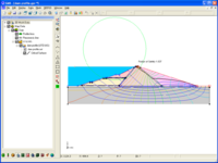
| <b>UTEXAS</b> is a slope stability software package created by Dr. Stephen G. Wright of the University of Texas at Austin. UTEXAS is used to analyze slope stability using the limit equilibrium method. The user provides the geometry and shear strength parameters for the slope in question and UTEXAS4 computes a factor of safety against slope failure. The factor of safety for a candidate failure surface is computed as the forces driving failure along the surface divided by the shear resistance of the soils along the surface. UTEXAS4 is a state-of-the-art slope stability code and has been widely used in industry for many years. | | <b>UTEXAS</b> is a slope stability software package created by Dr. Stephen G. Wright of the University of Texas at Austin. UTEXAS is used to analyze slope stability using the limit equilibrium method. The user provides the geometry and shear strength parameters for the slope in question and UTEXAS4 computes a factor of safety against slope failure. The factor of safety for a candidate failure surface is computed as the forces driving failure along the surface divided by the shear resistance of the soils along the surface. UTEXAS4 is a state-of-the-art slope stability code and has been widely used in industry for many years. |
|
| |
|
| GMS versions 6.5 and later include an interface to UTEXAS which allows users to create UTEXAS input files using GMS. | | GMS versions 6.5 and later include an interface to UTEXAS which allows users to create UTEXAS input files using GMS. |
| | |
| | The UTEXAS model can be added to a [http://www.aquaveo.com/software/gms-pricing paid edition] of GMS. |
| | [[Category:Link to Store]] |
|
| |
|
| ==Creating a Model== | | ==Creating a Model== |
| Existing UTEXAS models can be imported into GMS, or new models can be created from scratch. The UTEXAS interface is entirely within the [[GMS:Map Module|map module]]. The model consists of a [[GMS:Conceptual Model|conceptual model]] and one or more [[GMS:Coverages|coverages]]. | | Existing UTEXAS models can be imported into GMS, or new models can be created from scratch. The UTEXAS interface is entirely within the [[GMS:Map Module|map module]]. The model consists of a [[GMS:Conceptual Model|conceptual model]] and one or more [[GMS:Coverages|coverages]]. |
| *Importing | | *Importing |
| *:To import an existing UTEXAS model, use the standard '''''File|Open''''' command. The file to import is the UTEXAS input file. This file may have a "*.dat" extension which is (unfortunately) the extension UTEXAS expects. GMS creates the UTEXAS conceptual model and coverages from the file being imported. | | *:To import an existing UTEXAS model, use the standard ''File'' | '''Open''' command. The file to import is the UTEXAS input file. This file may have a *.dat extension which is (unfortunately) the extension UTEXAS expects. GMS creates the UTEXAS conceptual model and coverages from the file being imported. |
| *:Aspects of UTEXAS models can also be imported from a [[GMS:GeoStudio Import|GeoStudio]] file. | | *:Aspects of UTEXAS models can also be imported from a [[GMS:GeoStudio Import|GeoStudio]] file. |
| *Creating in GMS | | *Creating in GMS |
| Line 48: |
Line 53: |
|
| |
|
| ====Interpolated Pressure==== | | ====Interpolated Pressure==== |
| Another method for specifying the pore water pressure is "Pressure Interpolated" which uses a set of points where each point has a value representing the pore pressure at that point. In GMS, you can do this by associating a data set from a 2D mesh with the material. The data set might come from a [[GMS:SEEP2D|SEEP2D]] solution, since SEEP2D is a model in GMS that can solve for pore pressures. | | Another method for specifying the pore water pressure is "Pressure Interpolated" which uses a set of points where each point has a value representing the pore pressure at that point. In GMS, a user can do this by associating a dataset from a 2D mesh with the material. The dataset might come from a [[GMS:SEEP2D|SEEP2D]] solution, since SEEP2D is a model in GMS that can solve for pore pressures. |
|
| |
|
| ==Integration with SEEP2D== | | ==Integration with SEEP2D== |
| Line 62: |
Line 67: |
| To run UTEXAS: | | To run UTEXAS: |
|
| |
|
| * Export the model from GMS
| | # Export the model from GMS |
| * Launch UTEXAS (outside of GMS)
| | # Launch UTEXAS (outside of GMS) |
| * Open the exported file in UTEXAS
| | # Open the exported file in UTEXAS |
| * Wait for UTEXAS to finish
| | # Wait for UTEXAS to finish |
| * Read the solution into GMS
| | # Read the solution into GMS |
|
| |
|
| ===Exporting the Model=== | | ===Exporting the Model=== |
| To save a UTEXAS model that is in GMS in preparation for running UTEXAS, right-click on the UTEXAS model icon under the conceptual model and select the '''''Export''''' command. Note that GMS uses the extension *.utx instead of *.dat when saving the UTEXAS input file. | | To save a UTEXAS model that is in GMS in preparation for running UTEXAS, right-click on the UTEXAS model icon under the conceptual model and select the '''Export''' command. Note that GMS uses the extension *.utx instead of *.dat when saving the UTEXAS input file. |
|
| |
|
| ===Reading the Solution=== | | ===Reading the Solution=== |
| To read the solution generated by UTEXAS into GMS, right-click on the UTEXAS model icon under the conceptual model and select the '''''Read Solution''''' command. The UTEXAS solution will have an extension of '*.out'. | | To read the solution generated by UTEXAS into GMS, right-click on the UTEXAS model icon under the conceptual model and select the '''Read Solution''' command. The UTEXAS solution will have an extension of *.out. |
|
| |
|
| ==Display Options== | | ==Display Options== |
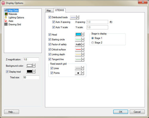
| A number of display options are associated with UTEXAS. To find these, select the '''Display Options''' button, click on the ''Map Data'' item from the list, and select the ''UTEXAS'' tab on the right. | | [[File:DisplayUTEXAS.jpg|thumb|500 px|The ''Display Options'' dialog showing the '' UTEXAS'' tab under the ''Map Data'' item.]] |
| | |
| | A number of display options are associated with UTEXAS. To find these, select the '''Display Options''' button, click on the ''Map Data'' item from the list, and select the ''UTEXAS'' tab on the right. The display options can also be accessed through the '''Display Options...''' command in the ''Display'' menu. |
|
| |
|
|
| |
|
| Line 84: |
Line 91: |
| | Distributed loads || Arcs that are designated as distributed loads. Arrows are drawn at the spacing and scale specified to show the loading. | | | Distributed loads || Arcs that are designated as distributed loads. Arrows are drawn at the spacing and scale specified to show the loading. |
| |- | | |- |
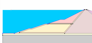
| | Head || [[Image:UtexasHeadDisplayOption.png|thumb|300px| ]] Arcs designated as Head arcs have the space above them filled with the specified color. | | | Head || [[Image:UtexasHeadDisplayOption.png|thumb|none|left|300px| ]] |
| | |
| | Arcs designated as Head arcs have the space above them filled with the specified color. |
| |- | | |- |
| | Starting circle || The starting circle specified in the ''UTEXAS Analysis Options'' dialog. | | | Starting circle || The starting circle specified in the ''UTEXAS Analysis Options'' dialog. |
| Line 94: |
Line 103: |
| | Limiting depth || The limiting depth specified in the ''UTEXAS Analysis Options'' dialog. | | | Limiting depth || The limiting depth specified in the ''UTEXAS Analysis Options'' dialog. |
| |- | | |- |
| | Tangent line || {{Version GMS 7.1}} The horizontal tangent line specified in the ''UTEXAS Analysis Options'' dialog. | | | Tangent line || The horizontal tangent line specified in the ''UTEXAS Analysis Options'' dialog. |
| |} | | |} |
| | |
| | ==UTEXAS Analysis Options== |
| | The ''UTEXAS Options'' dialog is reached though the ''UTEXAS'' | '''Analysis Options...''' menu command. |
| | [[File:UTEXASOptions.jpg|thumb|none|left|400 px|''UTEXAS Options'' dialog]] |
|
| |
|
| ==Unsupported Features== | | ==Unsupported Features== |
| Line 110: |
Line 123: |
|
| |
|
| ===Group B, Profile Lines=== | | ===Group B, Profile Lines=== |
| *Table 6.2, Group B - Profile Line Data Input Format - Import Mode | | *Table 6.2, Group B – Profile Line Data Input Format – Import Mode |
|
| |
|
| ===Group C, Material Properties=== | | ===Group C, Material Properties=== |
| *Table 7.1, Group C - Material Property Data Input Format | | *Table 7.1, Group C – Material Property Data Input Format |
| **Line 4 | | **Line 4 |
| ***Reference (R) | | ***Reference (R) |
| Line 122: |
Line 135: |
|
| |
|
| ===Group D, Piezometric Line=== | | ===Group D, Piezometric Line=== |
| *Table 8.1, Group D - Piezometric Line Data Input Format | | *Table 8.1, Group D – Piezometric Line Data Input Format |
| **Line 2 | | **Line 2 |
| ***Field 2, Unit weight of water | | ***Field 2, Unit weight of water |
|
| |
|
| ===Group E, Interpolation Data=== | | ===Group E, Interpolation Data=== |
| *Table 9.1 - GMS will export this table but cannot import it | | *Table 9.1 – GMS will export this table but cannot import it |
| *Table 9.2 - GMS won't import or export this table | | *Table 9.2 – GMS won't import or export this table |
|
| |
|
| ===Group G, Distributed Loads=== | | ===Group G, Distributed Loads=== |
| *Table 11.1, Group G - Distributed Load Data Input Format for Individual Points | | *Table 11.1, Group G – Distributed Load Data Input Format for Individual Points |
| **Line 2 | | **Line 2 |
| ***Field 4, Shear stress | | ***Field 4, Shear stress |
| Line 173: |
Line 186: |
| **UNS (Unsort) | | **UNS (Unsort) |
|
| |
|
| <h2>External Links</h2>
| | ==External Links== |
| * [ftp://pubftp.ems-i.com/download/GMS/GMS%206.5/models/UTEXAS4%20Manual.pdf UTEXAS4 Manual] | | * [ftp://pubftp.ems-i.com/download/GMS/GMS%206.5/models/UTEXAS4%20Manual.pdf UTEXAS4 Manual] |
| * [ftp://pubftp.ems-i.com/download/GMS/GMS%206.5/models/UTEXAS4%20Addendum.pdf UTEXAS4 Addendum] | | * [ftp://pubftp.ems-i.com/download/GMS/GMS%206.5/models/UTEXAS4%20Addendum.pdf UTEXAS4 Addendum] |
| Line 183: |
Line 196: |
| {{Navbox GMS}} | | {{Navbox GMS}} |
| [[Category:UTEXAS]] | | [[Category:UTEXAS]] |
| | [[Category:UTEXAS Dialogs]] |
| | [[Category:External Links]] |
| | [[Category:Archived]] |
UTEXAS is a slope stability software package created by Dr. Stephen G. Wright of the University of Texas at Austin. UTEXAS is used to analyze slope stability using the limit equilibrium method. The user provides the geometry and shear strength parameters for the slope in question and UTEXAS4 computes a factor of safety against slope failure. The factor of safety for a candidate failure surface is computed as the forces driving failure along the surface divided by the shear resistance of the soils along the surface. UTEXAS4 is a state-of-the-art slope stability code and has been widely used in industry for many years.
GMS versions 6.5 and later include an interface to UTEXAS which allows users to create UTEXAS input files using GMS.
The UTEXAS model can be added to a paid edition of GMS.
Creating a Model
Existing UTEXAS models can be imported into GMS, or new models can be created from scratch. The UTEXAS interface is entirely within the map module. The model consists of a conceptual model and one or more coverages.
- Importing
- To import an existing UTEXAS model, use the standard File | Open command. The file to import is the UTEXAS input file. This file may have a *.dat extension which is (unfortunately) the extension UTEXAS expects. GMS creates the UTEXAS conceptual model and coverages from the file being imported.
- Aspects of UTEXAS models can also be imported from a GeoStudio file.
- Creating in GMS
- Creating a UTEXAS model in GMS can be done a variety of ways. The UTEXAS tutorials illustrate these methods.
Profile Lines vs. Arcs and Polygons

Profile lines depicting a dam. Gaps show where lines begin and end (no gaps would exist in an actual model).
Profile Lines
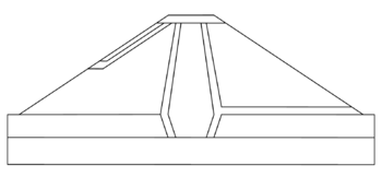
UTEXAS uses "profile lines" to define the soil stratigraphy. A profile line is a series of connected points that must go from left to right (or bottom to top) and represent the top of a soil layer. The profile line does not close on itself, and does not cross any other profile lines.
Polygons
GMS does not use profile lines, but instead uses arcs and polygons to define the soil stratigraphy. Using polygons is much easier than using profile lines because there is no need to worry about how to break up the lines such that they all go from left to right (or bottom to top).
When GMS saves the UTEXAS input file, it automatically figures out the profile lines that UTEXAS needs to represent the soil stratigraphy. When importing a UTEXAS file, GMS automatically builds arcs and polygons from the profile lines.
One notable difference between the profile line and polygon approaches is that when using polygons, the bottom-most polygon must be extended downward some distance below the bottom-most profile line to represent the bottom-most soil area.
Material Properties
UTEXAS soil material properties are entered in GMS using GMS materials. Each feature polygon has a material associated with it.
Pore Water Pressure
There are various ways to define pore water pressure. Two of the methods are more advanced: the piezometric line method, and the interpolated pressure method.
Piezometric Line
UTEXAS allows the pore water pressure to be specified using a piezometric line. In GMS, a piezometric line is an arc that is in it's own feature coverage (since the arc will likely overlap arcs in the profile line coverage). The material that uses the piezometric line can specify the coverage the piezometric line (arc) is in.
Interpolated Pressure
Another method for specifying the pore water pressure is "Pressure Interpolated" which uses a set of points where each point has a value representing the pore pressure at that point. In GMS, a user can do this by associating a dataset from a 2D mesh with the material. The dataset might come from a SEEP2D solution, since SEEP2D is a model in GMS that can solve for pore pressures.
Integration with SEEP2D
SEEP2D is a 2D seepage analysis model that, when combined with UTEXAS, provides a complete and a powerful 2D profile analysis solution. Since these two models are closely related, the conceptual model type for UTEXAS is called "SEEP2D/UTEXAS". One could use the same conceptual model to create both a SEEP2D model and a UTEXAS model. The UTEXAS tutorials illustrate this.
Running UTEXAS
UTEXAS differs from most models supported by GMS in the way that it is run. Most model codes supported by GMS can be run from inside GMS. Since UTEXAS is a Windows application with no command line options (yet), this is not possible.
Also, GMS typically provides a model wrapper
for most of the supported models as a convenient way to watch the progress of the model and automatically read in the results upon completion. Again, since UTEXAS is a Windows application, it is not possible to use a model wrapper.
To run UTEXAS:
- Export the model from GMS
- Launch UTEXAS (outside of GMS)
- Open the exported file in UTEXAS
- Wait for UTEXAS to finish
- Read the solution into GMS
Exporting the Model
To save a UTEXAS model that is in GMS in preparation for running UTEXAS, right-click on the UTEXAS model icon under the conceptual model and select the Export command. Note that GMS uses the extension *.utx instead of *.dat when saving the UTEXAS input file.
Reading the Solution
To read the solution generated by UTEXAS into GMS, right-click on the UTEXAS model icon under the conceptual model and select the Read Solution command. The UTEXAS solution will have an extension of *.out.
Display Options

The
Display Options dialog showing the
UTEXAS tab under the
Map Data item.
A number of display options are associated with UTEXAS. To find these, select the Display Options button, click on the Map Data item from the list, and select the UTEXAS tab on the right. The display options can also be accessed through the Display Options... command in the Display menu.
UTEXAS Display Options
| Option |
Description
|
| Distributed loads |
Arcs that are designated as distributed loads. Arrows are drawn at the spacing and scale specified to show the loading.
|
| Head |
Arcs designated as Head arcs have the space above them filled with the specified color.
|
| Starting circle |
The starting circle specified in the UTEXAS Analysis Options dialog.
|
| Factor of safety |
If a solution exists, the factor of safety.
|
| Critical surface |
If a solution exists, the critical surface.
|
| Limiting depth |
The limiting depth specified in the UTEXAS Analysis Options dialog.
|
| Tangent line |
The horizontal tangent line specified in the UTEXAS Analysis Options dialog.
|
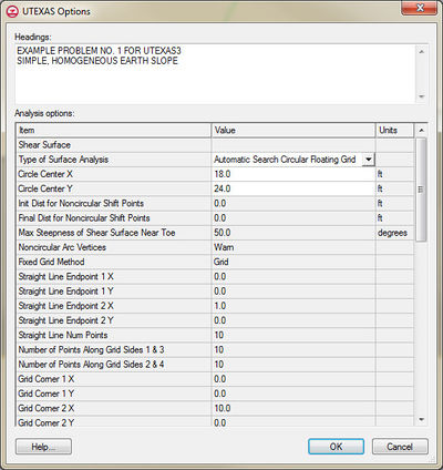
UTEXAS Analysis Options
The UTEXAS Options dialog is reached though the UTEXAS | Analysis Options... menu command.
Unsupported Features
Not all of the features of UTEXAS are currently supported in the GMS interface. Support for more features will be added in future versions of GMS. The following features are not supported.
Command Words
- LABel
- NO compute
- OTHer units
- SIUnits /or/ SI
- UT3
- UT4
- '***'
Group B, Profile Lines
- Table 6.2, Group B – Profile Line Data Input Format – Import Mode
Group C, Material Properties
- Table 7.1, Group C – Material Property Data Input Format
- Line 4
- Reference (R)
- Anisotropic shear (A)
- Interpolate Strengths (I S) (version 7.0 and earlier. Supported starting at GMS version 7.1)
- Line 6
- Interpolate Ru values (I R)
Group D, Piezometric Line
- Table 8.1, Group D – Piezometric Line Data Input Format
- Line 2
- Field 2, Unit weight of water
Group E, Interpolation Data
- Table 9.1 – GMS will export this table but cannot import it
- Table 9.2 – GMS won't import or export this table
Group G, Distributed Loads
- Table 11.1, Group G – Distributed Load Data Input Format for Individual Points
Group K, Analysis/Computation
- Table 14.2a
- Line 3
- Field 1, "T" (or "TANGENT") (version 7.0 and earlier. Supported starting at GMS version 7.1)
- Table 14.2c, "Fixed" Grid
- Line 3
- Field 1, "T" (or "TANGENT") (version 7.0 and earlier. Supported starting at GMS version 7.1)
- Table 14.2d, "Fixed" Grid
- Not supported in version 7.0 and earlier. Supported starting at GMS version 7.1. Also, although multiple criteria can be used to specify the radius, GMS only supports using one.
- Table 14.3, Summary of Sub-Command Words for Group K Data
- 1 (Same as "SIN" which GMS does support)
- 2 (Same as "TWO" which GMS does support)
- 3 (Same as "THR" which GMS does support)
- ARC (Arc length)
- BAS (Base length)
- CHA (Change)
- CRI (Critical shear surface)
- FAC (Factor of Safety)
- FOR (Force imbalance)
- INC (Increments for subdivision)
- ITE (Iteration)
- MIN (Minimum weight)
- MOM (Moment imbalance)
- PAS (Passes)
- RES (Restrictions)
- SAV (Save "n" most)
- SEI (Seismic coefficient) (version 7.0 and earlier. Supported starting at GMS version 7.1)
- SID (Side force inclination)
- SOR (Sort radii)
- STO (Stop)
- SUB (Subtended angle)
- TRI (Trial)
- UNI (Unit weight of water)
- UNS (Unsort)
External Links
