SMS:Inverse Distance Weighted Interpolation: Difference between revisions
| (37 intermediate revisions by 2 users not shown) | |||
| Line 1: | Line 1: | ||
One of the most commonly used techniques for interpolation of scatter points is inverse distance weighted (IDW) interpolation. Inverse distance weighted methods are based on the assumption that the interpolating surface should be influenced most by the nearby points and less by the more distant points. The interpolating surface is a weighted average of the scatter points and the weight assigned to each scatter point diminishes as the distance from the interpolation point to the scatter point increases. Several options are available for inverse distance weighted interpolation. The options are selected using the ''Inverse Distance Weighted Interpolation Options'' dialog. This dialog is accessed through the '''Options''' button next to the Inverse distance weighted item in the '' | One of the most commonly used techniques for interpolation of scatter points is inverse distance weighted (IDW) interpolation. Inverse distance weighted methods are based on the assumption that the interpolating surface should be influenced most by the nearby points and less by the more distant points. The interpolating surface is a weighted average of the scatter points and the weight assigned to each scatter point diminishes as the distance from the interpolation point to the scatter point increases. Several options are available for inverse distance weighted interpolation. The options are selected using the ''Inverse Distance Weighted Interpolation Options'' dialog. This dialog is accessed through the '''Options''' button next to the "Inverse distance weighted" item in the ''Interpolation'' dialog. SMS uses Shepard's Method for IDW: | ||
==Shepard's Method== | |||
The simplest form of inverse distance weighted interpolation is sometimes called "Shepard's method" (Shepard 1968). The equation used is as follows: | The simplest form of inverse distance weighted interpolation is sometimes called "Shepard's method" (Shepard 1968). The equation used is as follows: | ||
| Line 8: | Line 8: | ||
:<math>F(x,y) = \sum_{i=2}^n w_i f_i </math> | :<math>F(x,y) = \sum_{i=2}^n w_i f_i </math> | ||
where | :where ''n<'' is the number of scatter points in the set, ''f<sub>i</sub>'' are the prescribed function values at the scatter points (e.g. the dataset values), and ''w<sub>i</sub>'' are the weight functions assigned to each scatter point. The classical form of the weight function is: | ||
:<math>w_i = \frac {h_i^{-p}}{\displaystyle \sum_{j=i}^n h_j^{-p}} </math> | :<math>w_i = \frac {h_i^{-p}}{\displaystyle \sum_{j=i}^n h_j^{-p}} </math> | ||
where | :where ''p'' is an arbitrary positive real number called the power parameter (typically,''p=2'') and hi is the distance from the scatter point to the interpolation point or | ||
:<math>h_i = \sqrt{x-x_i)^2 + (y - y_i)^2}</math> | :<math>h_i = \sqrt{x-x_i)^2 + (y - y_i)^2}</math> | ||
where | :where ''(x,y)'' are the coordinates of the interpolation point and ''(x<sub>i</sub>,y<sub>i</sub>)'' are the coordinates of each scatter point. The weight function varies from a value of unity at the scatter point to a value approaching zero as the distance from the scatter point increases. The weight functions are normalized so that the weights sum to unity. | ||
The effect of the weight function is that the surface interpolates each scatter point and is influenced most strongly between scatter points by the points closest to the point being interpolated. | The effect of the weight function is that the surface interpolates each scatter point and is influenced most strongly between scatter points by the points closest to the point being interpolated. | ||
| Line 24: | Line 24: | ||
:<math> w_i = \frac {\left [ \frac {R - h_i}{Rh_i} \right ]^2}{\displaystyle \sum_{j=i}^n \left [ \frac {R-h_j}{Rh_j} \right ]^2 }</math> | :<math> w_i = \frac {\left [ \frac {R - h_i}{Rh_i} \right ]^2}{\displaystyle \sum_{j=i}^n \left [ \frac {R-h_j}{Rh_j} \right ]^2 }</math> | ||
where < | :where ''h<sub>i</sub>'' is the distance from the interpolation point to scatter point ''i'', ''R'' is the distance from the interpolation point to the most distant scatter point, and ''n'' is the total number of scatter points. This equation has been found to give superior results to the classical equation (Franke & Nielson, 1980). | ||
The weight function is a function of Euclidean distance and is radially symmetric about each scatter point. As a result, the interpolating surface is somewhat symmetric about each point and tends toward the mean value of the scatter points between the scatter points. Shepard's method has been used extensively because of its simplicity. | The weight function is a function of Euclidean distance and is radially symmetric about each scatter point. As a result, the interpolating surface is somewhat symmetric about each point and tends toward the mean value of the scatter points between the scatter points. Shepard's method has been used extensively because of its simplicity. | ||
== Computation of Nodal Function Coefficients == | == Computation of Nodal Function Coefficients == | ||
[[File:IDW Options.png|thumb|300 px|The ''IDW Options'' dialog]] | |||
In the ''IDW Interpolation Options'' dialog, an option is available for using a subset of the scatter points (as opposed to all of the available scatter points) in the computation of the nodal function coefficients and in the computation of the interpolation weights. Using a subset of the scatter points drops distant points from consideration since they are unlikely to have a large influence on the nodal function or on the interpolation weights. In addition, using a subset can speed up the computations since less points are involved. | |||
If the ''Use subset of points'' option is chosen, the '''Subsets''' button can be used to bring up the ''Subset Definition'' dialog. Two options are available for defining which points are included in the subset. In one case, only the nearest ''N'' points are used. In the other case, only the nearest ''N'' points in each quadrant are used as shown below. This approach may give better results if the scatter points tend to be clustered. | |||
:[[Image:Four_quadrants.jpg|thumb|none|left|200 px|The four quadrants surrounding an interpolation point.]] | |||
If a subset of the scatter point set is being used for interpolation, a scheme must be used to find the nearest ''N'' points. Two methods for finding a subset are provided in the ''Subset Definition'' dialog: the global method and the local method. | |||
;'''Global Method''' : With the global method, each of the scatter points in the set are searched for each interpolation point to determine which ''N'' points are nearest the interpolation point. This technique is fast for small scatter point sets but may be slow for large sets. | |||
;'''Local Method''' : With the local methods, the scatter points are triangulated to form a temporary TIN before the interpolation process begins. To compute the nearest ''N'' points, the triangle containing the interpolation point is found and the triangle topology is then used to sweep out from the interpolation point in a systematic fashion until the ''N'' nearest points are found. The local scheme is typically much faster than the global scheme for large scatter point sets. | |||
'''Local Method''' | |||
With the local methods, the scatter points are triangulated to form a temporary TIN before the interpolation process begins. To compute the nearest | |||
== Computation of Interpolation Weights == | == Computation of Interpolation Weights == | ||
| Line 53: | Line 46: | ||
When computing the interpolation weights, three options are available for determining which points are included in the subset of points used to compute the weights and perform the interpolation: subset, all points, and enclosing triangle. | When computing the interpolation weights, three options are available for determining which points are included in the subset of points used to compute the weights and perform the interpolation: subset, all points, and enclosing triangle. | ||
===Subset of Points=== | |||
If the Use subset of points option is chosen, the Subset Definition dialog can be used to define a local subset of points. | If the ''Use subset of points'' option is chosen, the ''Subset Definition'' dialog can be used to define a local subset of points. | ||
===All Points=== | |||
If the Use all points option is chosen, a weight is computed for each point and all points are used in the interpolation. | If the ''Use all points'' option is chosen, a weight is computed for each point and all points are used in the interpolation. | ||
===Enclosing Triangle=== | |||
The Use vertices of enclosing triangle method makes the interpolation process a local scheme by taking advantage of TIN topology (Franke & Nielson, 1980). With this technique, the subset of points used for interpolation consists of the three vertices of the triangle containing the interpolation point. The weight function or blending function assigned to each scatter point is a cubic S-shaped function as shown in part a of the figure below. The fact that the slope of the weight function tends to unity at its limits ensures that the slope of the interpolating surface is continuous across triangle boundaries. | The Use vertices of enclosing triangle method makes the interpolation process a local scheme by taking advantage of TIN topology (Franke & Nielson, 1980). With this technique, the subset of points used for interpolation consists of the three vertices of the triangle containing the interpolation point. The weight function or blending function assigned to each scatter point is a cubic S-shaped function as shown in part a of the figure below. The fact that the slope of the weight function tends to unity at its limits ensures that the slope of the interpolating surface is continuous across triangle boundaries. | ||
[[Image: | :[[Image:WMSidw_fig2.jpg|thumb|none|left|350 px|(a) S-shaped weight function and (b) Delauney point group for point A.]] | ||
The influence of the weight function extends over the limits of the Delauney point group of the scatter point. The Delauney point group is the "natural neighbors" of the scatter point, and the perimeter of the group is made up of the outer edges of the triangles that are connected to the scatter point as shown in part b. The weight function varies from a weight of unity at the scatter point to zero at the perimeter of the group. For every interpolation point in the interior of a triangle there are three nonzero weight functions (the weight functions of the three vertices of the triangle). For a triangle ''T'' with vertices ''i'', ''j'', and ''k'', the weights for each vertex are determined as follows: | |||
:<math>w_i (x,y) = b_i^2 (3 - 2b_i) + 3 \frac {b_i^2 b_j b_k}{b_i b_j + b_i b_k + b_j b_k} </math> | |||
:<math>\left \{ b_j \left [ \frac {| e_i |^2 + |e_k|^2 - | e_j |^2}{| e_k |^2} \right ] + b_k \left [ \frac {| e_i |^2 + | e_j |^2 - | e_k |^2}{| e_j |^2} \right ] \right \}</math> | |||
where || | :where ''||ei||'' is the length of the edge opposite vertex ''i'', and ''b<sub>i</sub>'', ''b<sub>j</sub>'', ''b<sub>k</sub>'' are the area coordinates of the point ''(x,y)'' with respect to triangle ''T''. Area coordinates are coordinates that describe the position of a point within the interior of a triangle relative to the vertices of the triangle. The coordinates are based solely on the geometry of the triangle. Area coordinates are sometimes called "barycentric coordinates." The relative magnitude of the coordinates corresponds to area ratios as shown below: | ||
:[[Image:WMSidw_fig3.jpg|thumb|none|left|400 px|Barycentric coordinates for a point in a triangle.]] | |||
The XY coordinates of the interior point can be written in terms of the XY coordinates of the vertices using the area coordinates as follows: | The XY coordinates of the interior point can be written in terms of the XY coordinates of the vertices using the area coordinates as follows: | ||
:<math>x = b_i x_i + b_j x_j + b_k x_k^{} </math> | |||
: | :<math>y = b_i y_i + b_j y_j + b_k y_k^{} </math> | ||
:<math>1.0 = b_i + b_j + b_k^{} </math> | |||
: | Solving the above equations for ''b<sub>i</sub>'', ''b<sub>j</sub>'', and ''b<sub>k</sub>'' yields: | ||
:[ | :<math>b_i \frac {1}{2A} [(x_j y_k - x_k y_j) + (y_j - y_k)x + (x_k - x_j)y]</math> | ||
:[ | :<math> b_j \frac {1}{2A} [ (x_k y_i - x_i y_k) + (y_k - y_i) x + (x_i - x_k) y]</math> | ||
:[ | :<math> b_k \frac {1}{2A} [ (x_i y_j - x_j y_i) + (y_i - y_j) x + (x_j - x_i) y]</math> | ||
:<math>A = \frac {1}{2} (x_i y_j + x_j y_k + x_k y_i - y_i x_j - y_j x_k - y_k x_i) </math> | |||
Using the weight functions defined above, the interpolating surface at points inside a triangle is computed as: | Using the weight functions defined above, the interpolating surface at points inside a triangle is computed as: | ||
:<math> F(x,y) = w_i (x,y) Q_i (x,y) + w_j (x,y) Q_j (x,y) + w_k (x,y) Q_k^{} (x,y) </math> | |||
: | :where ''w<sub>i</sub>'', ''w<sub>j</sub>'', and ''w<sub>k</sub>'' are the weight functions and ''Q<sub>i</sub>'', ''Q<sub>j</sub>'', and ''Q<sub>k</sub>'' are the nodal functions for the three vertices of the triangle. | ||
==Interpolate Inverse Distance Weighted Dialog== | |||
[[File:SMS-Interpolate-IDW.png|thumb|320 px|''Interpolate – Inverse Distance Weighted'' dialog]] | |||
The ''Interpolate – Inverse Distance Weighted'' dialog is reached from the [[SMS:Scatter_Interpolation#Interpolation_Options_Dialog|''Interpolation Options'']] dialog. It contains the following options: | |||
*''Computation of interpolation weights'' | |||
**''Use nearest'' – Drops points that are further than the indicated value. | |||
**''in each quadrant'' – When turned on, the nearest points in each quadrant are used in the subset. | |||
**''Use all points'' – All points will be used in the computation. | |||
*''Truncate values'' – This section allows for limiting the interpolated values to lie between the minimum and maximum value. | |||
**''Truncate to min/max of dataset'' – Limits the interpolated values to the minimum and maximum values in the original dataset. | |||
**''truncate to specified range'' – Allows setting a user specified minimum and maximum value range. | |||
***''Min'' – Manually sets a minimum value. | |||
***''Max'' – Manually sets a maximum value. | |||
==Related Topics== | |||
*[[SMS:Scatter Interpolation|Scatter Interpolation]] | |||
{{Template:Navbox SMS}} | |||
[[Category:SMS Interpolation|I]] | |||
[[Category:Interpolation Dialogs|I]] | |||
[[Category:Equations|I]] | |||
Latest revision as of 16:14, 15 October 2019
One of the most commonly used techniques for interpolation of scatter points is inverse distance weighted (IDW) interpolation. Inverse distance weighted methods are based on the assumption that the interpolating surface should be influenced most by the nearby points and less by the more distant points. The interpolating surface is a weighted average of the scatter points and the weight assigned to each scatter point diminishes as the distance from the interpolation point to the scatter point increases. Several options are available for inverse distance weighted interpolation. The options are selected using the Inverse Distance Weighted Interpolation Options dialog. This dialog is accessed through the Options button next to the "Inverse distance weighted" item in the Interpolation dialog. SMS uses Shepard's Method for IDW:
Shepard's Method
The simplest form of inverse distance weighted interpolation is sometimes called "Shepard's method" (Shepard 1968). The equation used is as follows:
- where n< is the number of scatter points in the set, fi are the prescribed function values at the scatter points (e.g. the dataset values), and wi are the weight functions assigned to each scatter point. The classical form of the weight function is:
- where p is an arbitrary positive real number called the power parameter (typically,p=2) and hi is the distance from the scatter point to the interpolation point or
- where (x,y) are the coordinates of the interpolation point and (xi,yi) are the coordinates of each scatter point. The weight function varies from a value of unity at the scatter point to a value approaching zero as the distance from the scatter point increases. The weight functions are normalized so that the weights sum to unity.
The effect of the weight function is that the surface interpolates each scatter point and is influenced most strongly between scatter points by the points closest to the point being interpolated.
Although the weight function shown above is the classical form of the weight function in inverse distance weighted interpolation, the following equation is used in SMS:
- where hi is the distance from the interpolation point to scatter point i, R is the distance from the interpolation point to the most distant scatter point, and n is the total number of scatter points. This equation has been found to give superior results to the classical equation (Franke & Nielson, 1980).
The weight function is a function of Euclidean distance and is radially symmetric about each scatter point. As a result, the interpolating surface is somewhat symmetric about each point and tends toward the mean value of the scatter points between the scatter points. Shepard's method has been used extensively because of its simplicity.
Computation of Nodal Function Coefficients
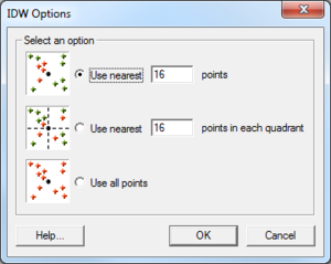
In the IDW Interpolation Options dialog, an option is available for using a subset of the scatter points (as opposed to all of the available scatter points) in the computation of the nodal function coefficients and in the computation of the interpolation weights. Using a subset of the scatter points drops distant points from consideration since they are unlikely to have a large influence on the nodal function or on the interpolation weights. In addition, using a subset can speed up the computations since less points are involved.
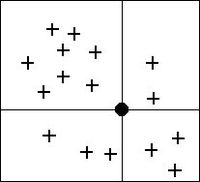
If the Use subset of points option is chosen, the Subsets button can be used to bring up the Subset Definition dialog. Two options are available for defining which points are included in the subset. In one case, only the nearest N points are used. In the other case, only the nearest N points in each quadrant are used as shown below. This approach may give better results if the scatter points tend to be clustered.
If a subset of the scatter point set is being used for interpolation, a scheme must be used to find the nearest N points. Two methods for finding a subset are provided in the Subset Definition dialog: the global method and the local method.
- Global Method
- With the global method, each of the scatter points in the set are searched for each interpolation point to determine which N points are nearest the interpolation point. This technique is fast for small scatter point sets but may be slow for large sets.
- Local Method
- With the local methods, the scatter points are triangulated to form a temporary TIN before the interpolation process begins. To compute the nearest N points, the triangle containing the interpolation point is found and the triangle topology is then used to sweep out from the interpolation point in a systematic fashion until the N nearest points are found. The local scheme is typically much faster than the global scheme for large scatter point sets.
Computation of Interpolation Weights
When computing the interpolation weights, three options are available for determining which points are included in the subset of points used to compute the weights and perform the interpolation: subset, all points, and enclosing triangle.
Subset of Points
If the Use subset of points option is chosen, the Subset Definition dialog can be used to define a local subset of points.
All Points
If the Use all points option is chosen, a weight is computed for each point and all points are used in the interpolation.
Enclosing Triangle
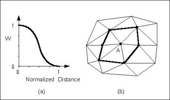
The Use vertices of enclosing triangle method makes the interpolation process a local scheme by taking advantage of TIN topology (Franke & Nielson, 1980). With this technique, the subset of points used for interpolation consists of the three vertices of the triangle containing the interpolation point. The weight function or blending function assigned to each scatter point is a cubic S-shaped function as shown in part a of the figure below. The fact that the slope of the weight function tends to unity at its limits ensures that the slope of the interpolating surface is continuous across triangle boundaries.
The influence of the weight function extends over the limits of the Delauney point group of the scatter point. The Delauney point group is the "natural neighbors" of the scatter point, and the perimeter of the group is made up of the outer edges of the triangles that are connected to the scatter point as shown in part b. The weight function varies from a weight of unity at the scatter point to zero at the perimeter of the group. For every interpolation point in the interior of a triangle there are three nonzero weight functions (the weight functions of the three vertices of the triangle). For a triangle T with vertices i, j, and k, the weights for each vertex are determined as follows:
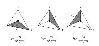
- where ||ei|| is the length of the edge opposite vertex i, and bi, bj, bk are the area coordinates of the point (x,y) with respect to triangle T. Area coordinates are coordinates that describe the position of a point within the interior of a triangle relative to the vertices of the triangle. The coordinates are based solely on the geometry of the triangle. Area coordinates are sometimes called "barycentric coordinates." The relative magnitude of the coordinates corresponds to area ratios as shown below:
The XY coordinates of the interior point can be written in terms of the XY coordinates of the vertices using the area coordinates as follows:
Solving the above equations for bi, bj, and bk yields:
Using the weight functions defined above, the interpolating surface at points inside a triangle is computed as:
- where wi, wj, and wk are the weight functions and Qi, Qj, and Qk are the nodal functions for the three vertices of the triangle.
Interpolate Inverse Distance Weighted Dialog
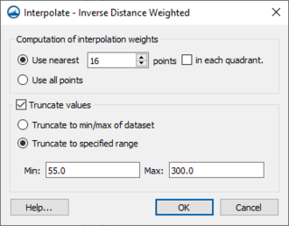
The Interpolate – Inverse Distance Weighted dialog is reached from the Interpolation Options dialog. It contains the following options:
- Computation of interpolation weights
- Use nearest – Drops points that are further than the indicated value.
- in each quadrant – When turned on, the nearest points in each quadrant are used in the subset.
- Use all points – All points will be used in the computation.
- Truncate values – This section allows for limiting the interpolated values to lie between the minimum and maximum value.
- Truncate to min/max of dataset – Limits the interpolated values to the minimum and maximum values in the original dataset.
- truncate to specified range – Allows setting a user specified minimum and maximum value range.
- Min – Manually sets a minimum value.
- Max – Manually sets a maximum value.
Related Topics
SMS – Surface-water Modeling System | ||
|---|---|---|
| Modules: | 1D Grid • Cartesian Grid • Curvilinear Grid • GIS • Map • Mesh • Particle • Quadtree • Raster • Scatter • UGrid |  |
| General Models: | 3D Structure • FVCOM • Generic • PTM | |
| Coastal Models: | ADCIRC • BOUSS-2D • CGWAVE • CMS-Flow • CMS-Wave • GenCade • STWAVE • WAM | |
| Riverine/Estuarine Models: | AdH • HEC-RAS • HYDRO AS-2D • RMA2 • RMA4 • SRH-2D • TUFLOW • TUFLOW FV | |
| Aquaveo • SMS Tutorials • SMS Workflows | ||


![{\displaystyle w_{i}={\frac {\left[{\frac {R-h_{i}}{Rh_{i}}}\right]^{2}}{\displaystyle \sum _{j=i}^{n}\left[{\frac {R-h_{j}}{Rh_{j}}}\right]^{2}}}}](https://en.wikipedia.org/api/rest_v1/media/math/render/svg/d4135f6bba53b4103d976f258474112e870d90c6)

![{\displaystyle \left\{b_{j}\left[{\frac {|e_{i}|^{2}+|e_{k}|^{2}-|e_{j}|^{2}}{|e_{k}|^{2}}}\right]+b_{k}\left[{\frac {|e_{i}|^{2}+|e_{j}|^{2}-|e_{k}|^{2}}{|e_{j}|^{2}}}\right]\right\}}](https://en.wikipedia.org/api/rest_v1/media/math/render/svg/bfb7e83454656986450660492722c205b045e194)


![{\displaystyle b_{i}{\frac {1}{2A}}[(x_{j}y_{k}-x_{k}y_{j})+(y_{j}-y_{k})x+(x_{k}-x_{j})y]}](https://en.wikipedia.org/api/rest_v1/media/math/render/svg/1b3e45440623afce692f1154d13fec76cd93339f)
![{\displaystyle b_{j}{\frac {1}{2A}}[(x_{k}y_{i}-x_{i}y_{k})+(y_{k}-y_{i})x+(x_{i}-x_{k})y]}](https://en.wikipedia.org/api/rest_v1/media/math/render/svg/40a2b23468b1457c72cdb837a616d8ebba1d27dc)
![{\displaystyle b_{k}{\frac {1}{2A}}[(x_{i}y_{j}-x_{j}y_{i})+(y_{i}-y_{j})x+(x_{j}-x_{i})y]}](https://en.wikipedia.org/api/rest_v1/media/math/render/svg/adbd5c97966c6b5e760f74b572c0e98834d1af34)


