UGrids Tools
This article describes tools from the SMS toolbox that are used to edit, create, and otherwise modify UGrids.
UGrids Tools
Convert to Voronoi UGrid
The Convert to Voronoi UGrid tool creates a Voronoi UGrid from an existing geometry (2D Mesh, Scatter Set, or UGrid). The tool uses the centroid of each triangle, element or cell of the input geometry as a node in the resulting Voronoi UGrid. The cells around the edge of the UGrid are created by adding a Voronoi node at the bisection of the boundary edge and connecting that node to the node at the triangle/element/cell centroid.
These meshes can be passed into HEC-RAS 2D for analysis.
Input parameters
- Input grid – Select the geometry that will be converted to a Voronoi UGrid.
Output parameters
- Output grid name – Enter the name for the new Voronoi UGrid. This will be a UGrid because scatter sets and meshes do not support polygonal cells.
Current Location in toolbox
Unstructured Grids/Convert to Voronoi UGrid
Convert 3D Data to 2D Data
The Convert 3D Data to 2D Data tool is used to convert 3D cell data to a 2D UGrid with datasets. The user selects a 3D cell dataset as input to the tool (the dataset may have multiple time steps). Then the user may choose to output multiple datasets from the tool; the following datasets may be computed by the tool: highest active value, average, maximum, minimum, value for each layer. The 3D UGrid cells are organized into columns of cells to compute the various output datasets. Examples follow that explain how the tool works for different types of UGrids. This tool will only work on UGrids that are made up of 3D cells and those cells must all be prisms (the side faces of the cells must be vertical). Further, the grid must have layers assigned to the cells. The tool will return an error if any of these conditions are not met.
Input parameters
- Cell dataset – The input 3D dataset that will be converted to 2D datasets
- Name of the output grid – Name for the newly created 2D UGrid. If this value is left blank then the name of the output grid will be set to be the name of the input cell dataset.
- Compute highest active cell in column – Option to output a 2D dataset where the value will come from the highest active cell in the 3D column of cells.
- Compute average value in column – Option to output a 2D dataset of the average value in the 3D column of cells.
- Compute maximum value in column – Option to output a 2D dataset of the maximum value in the 3D column of cells.
- Compute minimum value in column – Option to output a 2D dataset of the minimum value in the 3D column of cells.
- Compute value for each layer in column – Option to output 2D datasets of the value for each layer in the 3D column of cells.
Output parameters
- The output is a 2D UGrid and datasets.
Current location in Toolbox
Unstructured Grids/Convert 3D Data to 2D Data
Examples
Files for example 1 and example 3 can be downloaded here.
Example 1
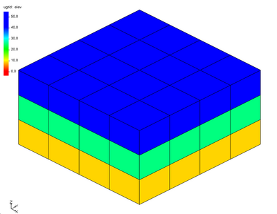
The first example is a simple structured 3D Grid. The grid is made up of 4 rows, 4 columns, and 3 layers.
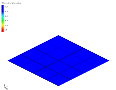
The dataset “elev” has constant values for each layer of the grid: layer 1 – 41.6, layer 2 – 25.0, and layer 3 – 8.3. Running the tool on this dataset produces the following 2D UGrid and datasets.
In this example the datasets are straight forward.
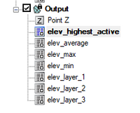
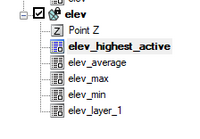
The "elev_highest_active" creates a dataset with values from the top of the 3D UGrid. All of the values are 41.6. The "elev_average" dataset gives the average value in each cell column and in this case that will match the values from layer 2 of the 3D UGrid (25.0). The elev_max dataset matches the values of the top layer of the 3D UGrid (41.6). The "elev_min" dataset matches the values from the bottom layer of the 3D UGrid (8.3). The "elev_layer_1", "elev_layer_2", and "elev_layer_3" match the values from the respective layer of the 3D UGrid.
Example 2
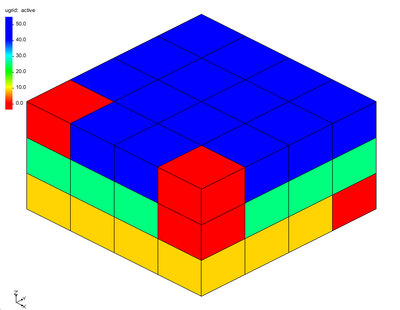
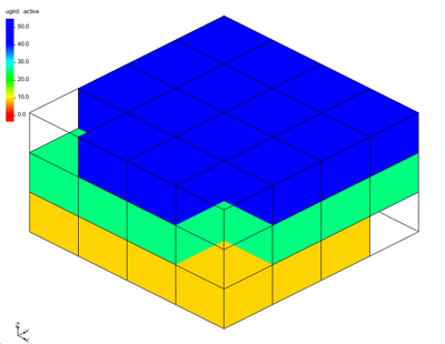
The second example is the same 3D Grid from example 1 except in this case the 3D dataset has activity. That is to say, some of the values in the dataset are considered inactive. The cells with inactive values are shown in red in the following figure.
Typically, these values are not contoured on the 3D UGrid.
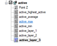
When the tool runs with this example the following datasets are created. First, examine the layer datasets and notice the effect that activity has on the created datasets.
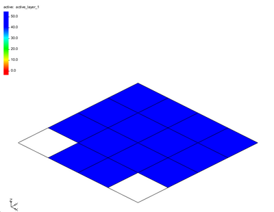
The "active_layer_1" dataset shows the 2 cells with inactive values.
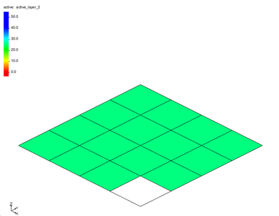
The "active_layer_2" dataset show the 1 cell with an inactive value.
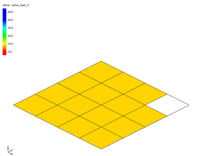
The "active_layer_3" dataset shows the 1 cell with an inactive value.
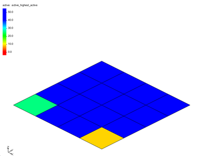
The "active_highest_active" has values from 2 of the lower layers in the 3D UGrid.
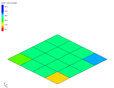
The "active_average" has 3 values that are affected by the dataset activity. The "active_maximum" and "active_minimum" datasets are similar to the "active_average".
Example 3
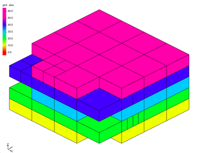
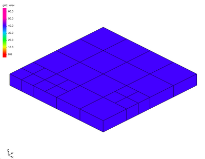
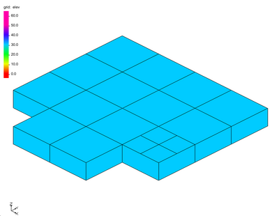
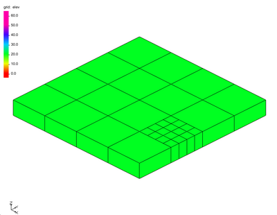
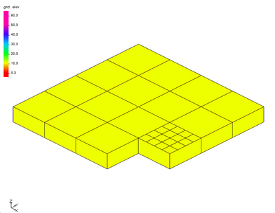
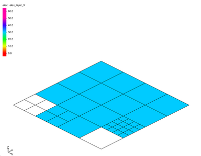
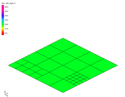
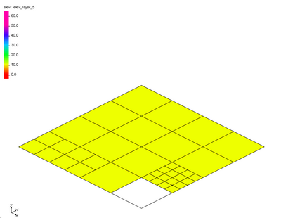
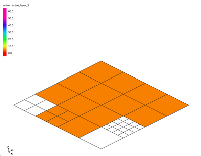
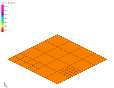
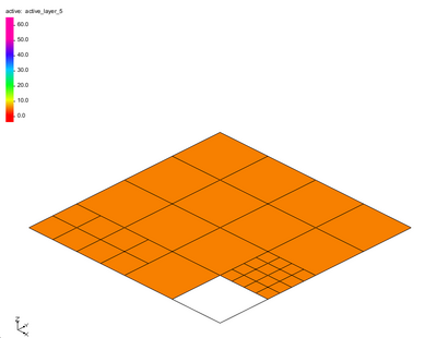
The third example is a 3D UGrid with variable number of cells per layer and variable refinement in each layer. A figure of the entire grid is shown, followed by figures of individual layers.
Layer 2 of the 3D UGrid:
Layer 3 of the 3D UGrid:
Layer 4 of the 3D UGrid:
Layer 5 of the 3D UGrid:
When the tool is run with this example the following datasets are created.
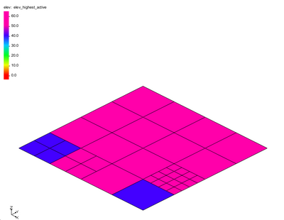
The next figure shows the resulting 2D UGrid with the "elev_highest_active" dataset contoured.
Notice that the 2D cells are defined by the smallest 3D cells in any column. The 2 cells that are not pink have values that came from layer 2 of the 3D Grid. The "elev_average", "elev_maximum", "elev_minimum" are computed in a straight forward manner and are not shown here.
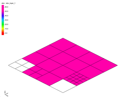
The "elev_layer" datasets are shown next. Notice that some layer datasets have inactive values because there were no cells defined in those cell columns.
The "elev_layer_1" dataset:
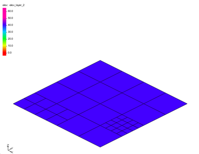
The "elev_layer_2" dataset:
The "elev_layer_3" dataset:
The "elev_layer_4" dataset:
The "elev_layer_5" dataset:
Example 4
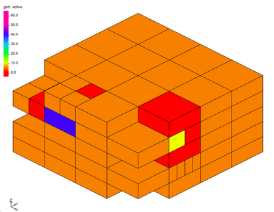
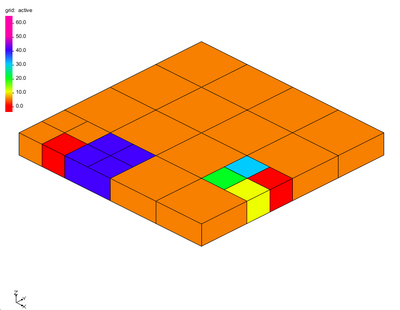
The fourth example uses the same 3D UGrid as example 3 and the dataset now includes activity. The orange cells in the grid have a value of 5. The red cells have inactive dataset values.
Layer 2 values for 3D UGrid:
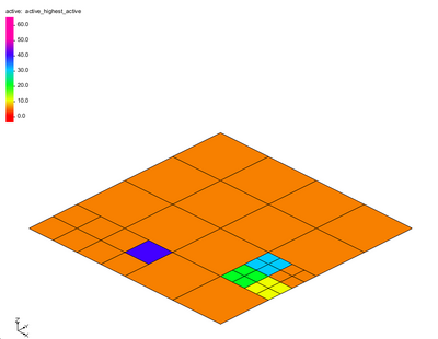
When the tool is executed the following results are generated from the tool.
The "active_highest_active" dataset result:
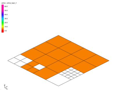
The "active_layer_1" dataset:
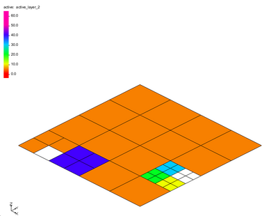
The "active_layer_2" dataset:
The "active_layer_3" dataset:
The "active_layer_4" dataset:
The "active_layer_5" dataset:
Example 5
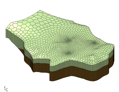
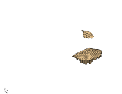
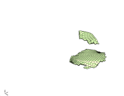
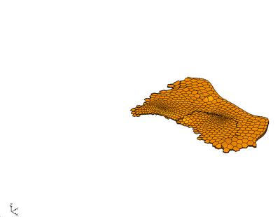
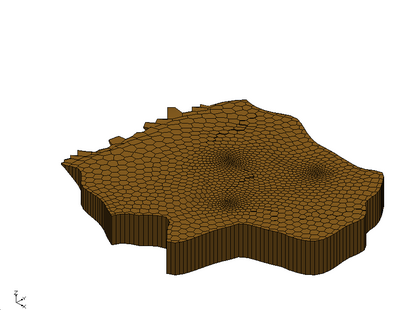
The fifth example is a voronoi 3D UGrid. This grid has a variable number of cells in each layer. This example comes from the MODFLOW-USG Complex Stratigraphy tutorial.
Layer 2 of 3D UGrid:
Layer 3 of 3D UGrid:
Layer 4 of 3D UGrid:
Layer 5 of 3D UGrid:
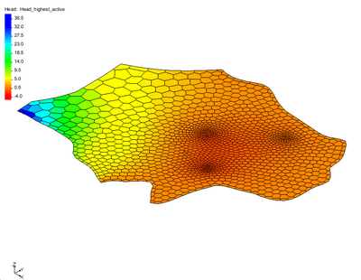
When the tool is run the following figure shows the output 2D UGrid:
Convert Mesh/Scatter/Cartesian Grid to UGrid
The tool creates a new UGrid with copies of all of the datasets on the input mesh, scatter set, or Cartesian grid.
Input parameters
- Input grid – Select the input mesh, scatter set, or Cartesian grid to convert to a UGrid.
Output parameters
- Output grid name – Enter the name of the new Ugrid. If left blank the tool will use the name of the input UGrid.
Current location in Toolbox
Unstructured Grids/Convert Mesh/Scatter/Cartesian Grid to UGrid
Convert to 2D Mesh
The tool creates a new 2D mesh with copies of all of the datasets associated with the input Ugrid.
Input parameters
- 2D UGrid – Select the input UGrid to convert to a 2D mesh.
- Create from – Indicates whether to use the UGrid cell centers or points for the nodes of the mesh.
- "UGrid cell centers" – This option will use the cell centers of the UGrid elements as the nodes for the mesh.
- "Ugrid points" – This option will use the UGrid points as the nodes for the mesh.
Output parameters
- Mesh name – Enter the name of the new mesh. If left blank the tool will use the name of the input UGrid.
Current location in Toolbox
Unstructured Grids/Convert to 2D Mesh
Create Bridge Footprint
The Create Bridge Footprint tool can be used to assist in the creation of an unstructured mesh under and around a bridge structure. Meshing this portion of a domain can lead to complexity. By the nature of the region, flow is complex due to contractions, obstructions and local flow patterns around piers and abutments. When water levels are high enough to induce pressure flow, the constraints on meshing are even more critical.
Some models, such as SRH-2D are more stable when the elements just upstream and downstream of the transitions into and out of pressure flow are rectangular elements aligned to the flow. Further, wrapping structures such as piers with small elements transitioning to larger elements has traditionally required many polygons in a Mesh Generation Coverage.
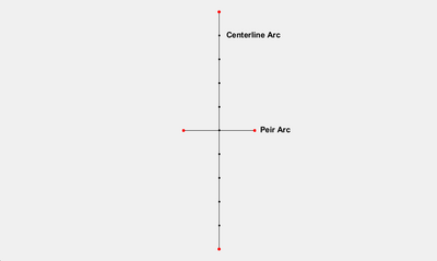
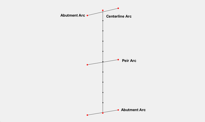
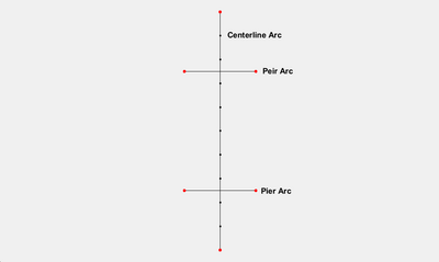
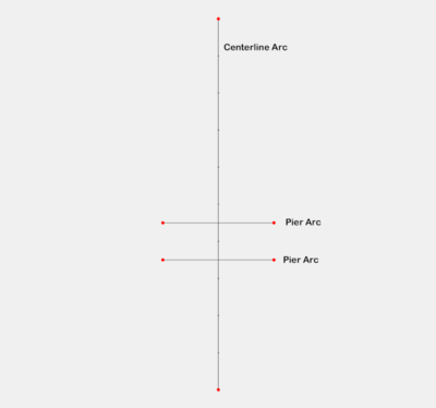
The Create Bridge Footprint tool requires a definition of a bridge footprint to be provided generically in any coverage type. This definition consists of:
- An arc along the centerline of the bridge. The distribution of vertices on the centerline affects the number of elements created.
- Arcs crossing the centerline (but not intersecting at a node) at the location of each pier (wall pier or pier group.
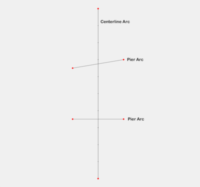
- Arcs crossing the centerline near the end defining the orientation of the bridge abutments if these abutments are not perpendicular to the centerline.
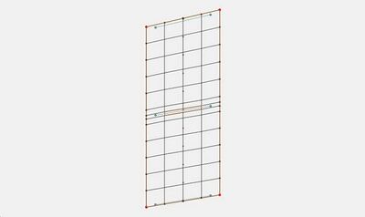
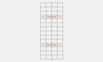
The tool creates a coverage that bounds the area of the bridge that can be incorporated into a Mesh Generation Coverage of the simulation domain along with a mesh that represents the area under and around the bridge.
Input parameters
- Input coverage – This can be any coverage but it represents a single bridge. The coverage will have no polygons or feature points (points that are not part of any arcs). The longest arc is interpreted as the bridge centerline. All other arcs in the coverage should cross, but not intersect this arc (intersecting would result in splitting both arcs). All other arcs (which cross the bridge centerline) are assumed to define the location of a wall pier or pier group, unless the "Has abutments" toggle is selected. In this case, the arcs that intersect the centerline closest to the ends of the centerline arc define the orientation of the bridge abutments at the ends of the centerline. See the figure in the examples below.
- Bridge width – Enter the total width of the bridge from upstream face to downstream face. The units (foot/meter) correspond to the display projection of SMS.
- Bridge wrapping width – Enter the width of a rows of cells created just upstream and just downstream of the bridge footprint. These will be quadrilateral cells to cleanly represent the flow entering/leaving the bridge region. This width is usually specified to transition from smaller cells under the bridge to larger/longer cells in the channels upstream and downstream of the bridge.
- Specify number of segments (toggle) – This allows the user to define a number of segments in the wrapping layer. Normally this number comes from the number of elements representing the bridge cross section (spacing on the centerline arc and number of piers). If the number of elements in the bridge cross section is significantly different from the number of elements in the channel, this option can be used to provide a transition.
- Has abutments (toggle) – Setting this option instructs the tool to interpret the first and last crossing arcs as abutment orientations. If the toggle is not selected, the abutments are created perpendicular to the bridge centerline.
- Pier type – Specify that the piers in this bridge will be wall piers or pier groups (mixed types of piers in a single bridge are not currently supported).
- Wall width (option for wall piers) – Enter the width of the wall piers.
- Element wrapping width (option for wall piers) – Enter the desired width of the element adjacent to the pier. It is expected that this will normally be a small value to represent the boundary layer next to the pier. The tool will transition from this width to the spacing along the centerline.
- Wall pier length (option for wall piers) – Enter the length of the wall piers (in direction of flow). (The length of the arcs is not important.)
- Wall pier number of side elements (option for wall piers) – Enter the number of elements that should be created in the direction of flow alongside the wall pier.
- Pier end type - Square/Round/Sharp (option for wall piers) – Enter the resolution for the end of the pier. Square puts 1 element/cell on the end of the pier, sharp puts 2, round puts 3. Normally "Square" results are sufficient.
- Pier diameter (option for pier groups) – Enter the diameter of the piers. (All piers currently have the same diameter.)
- Element wrapping width (option for pier groups) – Enter the desired width of the element adjacent to the pier. It is expected that this will normally be a small value to represent the boundary layer next to the pier. The tool will transition from this width to the spacing along the centerline.
- Number of piers in group (option for pier groups) – Enter an integer number of piers in a group.
- Pier group spacing (option for pier groups – Enter the distance (centroid to centroid) between piers in a pier group.
Output parameters
- Output grid – Enter the name of the grid to be created (representing the area under the bridge).
- Output coverage – Enter the name of the coverage to be created (representing the bridge footprint). The intent of this coverage is to incorporate this polygon into the mesh generation coverage for the simulation domain and define transition from the channels and embankments into the bridge region.
Current Location in toolbox
Unstructured Grids/Create Bridge Footprint
Examples
Example 1 – Simple Bridge with a Single Pier
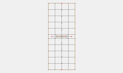
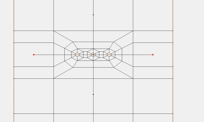
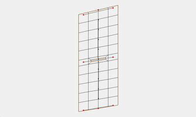
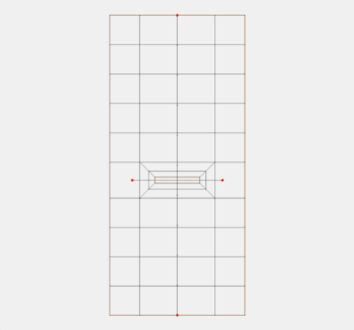
In this case the bridge width was set to 20.0, the wrapping width to 10.0. The pier is a wall pier with a width of 2, a wrapping width of 2 and a length of 15.0. Notice that the resulting elements above and below the pier do not line up with the vertices on the centerline arc. The vertices on the centerline arc are used to determine the number of segments between each pier and the segements are equally spaced between piers.
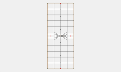
The next figure show a mesh where the pier type was changed to a pier group.
Zoomed in on the group
Example 2 – Bridge with Abutments and a Skewed Pier
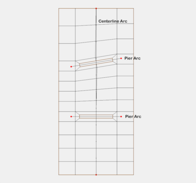
In this case the bridge width was set to 20.0, the wrapping width to 10.0. The pier is a wall pier with a width of 2, a wrapping width of 2 and a length of 15.0. The “Has abutments” option was turned on. The skew of the pier and the abutments is parallel to the lines defining those features.
Example 3 – Box Culvert
This tool can also be used to insert a box culvert. Using the same coverage as the previous example, we will specify the pier length to be 20.0. This means the pier will intersect the bridge width. Whenever the length of the pier plus the wrapping width intersects the width of the bridge then the pier is treated like a wall in a box culvert. The next figure shows the resulting mesh.
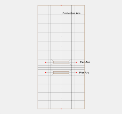
Example 4 – Multiple Piers
In this case the bridge width was set to 20.0, the wrapping width to 10.0. The pier is a wall pier with a width of 2, a wrapping width of 2 and a length of 15.0.
Example 5 – Multiple Piers 2
This is similar to the previous example except one of the piers is skewed.
In this case the bridge width was set to 20.0, the wrapping width to 10.0. The pier is a wall pier with a width of 2, a wrapping width of 2 and a length of 15.0. Notice that because of the skew the number of elements is different on the upstream and downstream faces of the mesh. This forces transition elements (triangles) where the number of elements changes.
Example 6 – Intersecting Piers
Sometimes piers may be close to one another as shown in the next example.
In this case the bridge width was set to 20.0, the wrapping width to 10.0. The pier is a wall pier with a width of 2, a wrapping width of 2 and a length of 10.0. With only the upper pier the mesh would look like the following figure.
When running the tool with both piers the tool will determine how large the piers can be without intersecting. Then another layer of elements will be placed between the piers and the bridge width.
The next figure shows the mesh with the bridge width reduced to 15.0 and wrapping width to 2.5 so that the final mesh has a width of 20.
Related Tools
Export Curvilinear Grid
The Export Curvilinear Grid tool is used to create a curvilinear (boundary fitted) grid file (or files) for a curvilinear compatible mesh, scatter set or UGrid that is loaded into SMS. This can make use of user provided I,J index data sets if they exist. It also supports the option to compute I,J data indices. In this case, the orientation of the first cell in the surface will define the orientation of the I,J axes of the grid.
For EFDC grid files it may also use provided cell based datasets to populate the additional properties of the grid. These can include:
- Depth
- Z Roughness
- Vegetation type
- Wind shelter
Input Parameters
The format of the data file will be in either CH3D (also referred to as GSMB) or EFDC (also referred to as LTFATE). The input parameters include:
- Generate cell i-j datasets toggle.
- Cell i-coordinate dataset (optional) – Select the cell based dataset that defines the I index of each cell. This is required if the toggle to generate I-J is not selected.
- Cell j-coordinate dataset (optional) – Select the cell based dataset that defines the J index of each cell. This is required if the toggle to generate I-J is not selected.
Datasets that are available if the format is EFDC:
- Depth dataset (optional) – Select the cell based dataset to define the depth of each cell.
- Z Roughness dataset (optional) – Select the cell based to define the roughness of each cell.
- Vegetation type dataset (optional) – Select the cell based to define the vegetation type of each cell.
- Wind shelter dataset (optional) – Select the cell based to define the wind shelter value of each cell.
Output Parameters
The path to where files will be saved defaults to the project directory if one is defined in the instance of SMS. The path can be cut/paste from a file browser in windows to this edit field.
- CH3D grid file name defaults to "grid.inp".
- EFDC dxdy file name defaults to "dxdy.inp".
- EFDC lxly file name defaults to "lxly.inp".
- EFDC cell file name defaults to "cell.inp".
Current location in toolbox
This tool is currently located in Unstructured Grids/Export Curvilinear Grid.
Notes
The file formats for the CH3D and EFDC grids are defined in the Import Curvilinear Tool documentation. The cell.inp file for EFDC is not used for importing since it does not include any unique information for the definition of the grid. This file includes an ASCII map of the cell types in the grid.
Import Curvilinear Grid
The Import Curvilinear Grid tool is used to load an existing curvilinear (boundary fitted) grid into SMS as a UGrid object. This will also create cell based datasets defining the I, J index of each cell in the UGrid. Depending on the selected format and the specific data file(s).
For EFDC grid files it may also create additional cell based datasets for the UGrid that is loaded. These can include:
- Depth
- Z Roughness
- Vegetation type
- Wind shelter
Input parameters
- Format of the data file – Select the file format for the UGrid that will be imported.
- "CH3D" – Will import a CH3D file.
- "EFDC" – Will import a EFDC file.
- CH3D formatted grid file – Clicking the Select File button will open a Select File dialog where the CH3D file can be selected.
- EFDC formatted dxdy.inp file – Clicking the Select File button will open a Select File dialog where the dxyy.inp EFDC file can be selected.
- EFDC formatted lxly.inp file – Clicking the Select File button will open a Select File dialog where the lxly.inp EFDC file can be selected.
Output parameters
- Output UGrid name – Enter the name of the imported UGrid.
Current location in the toolbox
Unstructured Grids/Import Curvilinear Grid
CH3D Format
Format of the CH3D file (grid.inp). This file includes a 2 line header and a line for every corner point in a rectangular grid This includes inactive regions. The locations are ordered in a row major order. SMS will export 5 columns of data including (X, Y, Z, I, J). The (I, J) columns are not used in the import process. They are implied. The first line is a name to assign to the grid.
The second line defines the size of the grid based on cell corners. The number of cells in each direction is a maximum of the number of corners minus 1. Cell corners that do not correspond to an active cell in the grid is assigned a coordinate location of (9.0x10¹⁸, 9.0x10¹⁸, 9.0x10¹⁸).
Because this file format does not include cell based information, a single row or column of inactive cells is not supported. The corners of these cells are defined by the active neighbor, so the cell is assumed to exist. File organization:
    Grid_name
    num_rows_of_pts  num_cols_of_pts
    x y z 1 1
    x y z 2 1
    .
    .
    .
    x y z num_rows 1
    x y z 1 2
    x y z 2 2
    .
    .
    .
    x y z num_rows 2
    .
    .
    .
    x y z 1 num
Format of the EFDC files (dxdy.inp, lxly.inp). This format includes two files that work together to define the grid. The "dxdy.inp" files includes a 4 line comment header and a line for every active cell in the grid The header is metadata only and is not used in the import process. The last header line defines the values in each column for the data following. This includes:
- I J: the column and row index of the cell on this line.
- DX DY: the width and height of this cell.
- WATER DEPTH: the depth of the water in this cell.
- BOTTOM ELEV: the ground elevation value for this cell (cell based).
- ZROUGH: the roughness for this cell.
- VEG TYPE: the vegetation type for this cell.
The "lxly.inp" files also includes a 4 line comment header and a line for every active cell in the grid The header is metadata only and is not used in the import process. The last header line defines the values in each column for the data following. This includes:
- I J: the column and row index of the cell on this line.
- X Y: the location of the cell center of this cell.
- CUE CVE CUN CVN: the orientation of this cell (rotation values)
- WIND SHELTER: a wind shelter data value for this cell.
This format defines a nonconformal grid. Neighboring cells don't explicitly define the same corner points. When SMS loads this grid, the corner locations are merged to create a conformal grid. For this reason, when a grid is loaded and then rewritten, the detail definition may not be identical.
Import UGrid Points
The Import UGrid Points tool is used to import locations and datasets. The CSV file must contain coordinates for the points and, optionally, the file may contain datasets associated with the points.
The first line of the CSV file must be a header line with the coordinate columns of x, y, and z (optional). These columns must be named x, y, z. An error will be encountered if these columns do not exist.
Other columns may exist in the file for datasets. The dataset name is specified in the first line of the file. If the column does not have a name then the column will be skipped.
Transient data may also be imported using this tool. Transient datasets comprise multiple columns in the file with the same column name and with time specified on the second line of the file in the associated dataset column. There may not be any value specified on the second line of the file for the x, y coordinates. The time values may be relative times: 0.0, 2.5, 10.0, etc. Additionally, the time values may be specified as date times. The date format should be in the form of YEAR-MONTH-DAY HH:MM:SS.SS.
Multiple example files are shown below.
Input parameters
- CSV file with point coordinates and datasets – Shows the file name for the CSV file containing the coordinates and datasets. Clicking the Select File button will open a Select File browser dialog to select the CSV file.
- No data value – When the “No data value” is encountered in the csv file in one of the datasets XMS marks the value as “NULL” or “no data”. These values are not contoured or used in interpolation in XMS.
- Time unit – The time unit for transient datasets where the time is specified as a floating point number (in contrast to a date time).
- Coordinate system project file (*.prj) – Shows the file name for the projection associated with the coordinates of the points in the file. Clicking the Select File button will open a Select File browser dialog to select the PRJ file.
Current location in Toolbox
Unstructured Grids/Import UGrid Points
Example files
Example 1
id,y,x,c
1,15459458,2685809,6.4
2,15459506,2685824,9.7
3,15459524,2685850,8
This is a simple csv file. Notice the “x” and “y” columns; these are required. Note that “z” is not required. Also, notice that the order of x and y does not matter.
The other 2 columns: “id”, “c”. The will be imported as datasets.
Example 2
y	x	z	TDS	TDS	conc
			0	1
-16	-75	8.5	59.04	9.24	1.9
32	-60	9.8	90.2	71	4.8
50	-34	0.7	67.2	98.4	9.5
This example shows a file with “x”, ”y”, and “z” columns. Notice that there are no values on the second line of the file for x, y, and z. This indicates that times are being specified for the datasets in the file.
The other 2 columns: “TDS” and “conc”. The will be imported as datasets. TDS will be a transient dataset with times of 0.0 and 1.0. The user will have to specify the units of the times in the tool. The conc dataset will be imported without multiple time steps.
Example 3
y	x	c2	c2	c2
		2011-02-01	2012-02-01	2013-02-01
-16	-75	59.04	43.64	9.24
32	-60	90.2	44.16	71
50	-34	67.2	0	98.4
This is a csv file with a transient dataset with the time specified as dates.
Example 4
y	X	c2	c2	c2
		2011-02-01 15:30:22.1	2012-02-01	2013-02-01 6:45:15
-16	-75	59.04	43.64	9.24
32	-60	90.2	44.16	71
50	-34	67.2	0	98.4
This is a csv file with a transient dataset with the time specified as dates and times.
Interpolate to UGrid
The Interpolate to Ugrid tool will interpolate a dataset associated with one UGrid to another UGrid within the same project.
Input Parameters
- Source dataset – Select the dataset that will be used for interpolation.
- Target grid – Select the grid that will be receiving the interpolated dataset.
- Target dataset name – Name of the target dataset.
- Target dataset location – Indicates if the dataset should be interpolated to the either the "Points" or the center of each "Cell" of the target grid.
- Interpolation method – The following interpolation methods are supported:
- "Linear" – Uses data points that are first triangulated to form a network of triangles.
- "Inverse Distance Weighted (IDW)" – Based on the assumption that the interpolating surface should be influenced most by the nearby points and less by the more distant points.
- "Natural Neighbor" – Based on the Thiessen polygon network of the point data.
- Interpolation dimension – Set be either "2D" or "3D" interpolation. Should match the target grid's dimensions.
- Truncate interpolated values option – The interpolated values can be limited by using one of the following truncation options:
- "Do not truncate" – Interpolated values will not be truncated.
- "Truncate to min/max of source dataset" – Interpolated values will be restricted to the minimum and maximum values in the source dataset.
- "Truncate to specified min/max" – Interpolated values will be restricted to a define minimum and maximum value.
- Truncate range minimum – Define the minimum value for truncating.
- Truncate range maximum – Define the maximum value for truncating.
- IDW nodal function – Available when using the IDW interpolation method. Select an IDW nodal function method using one of the following:
- "Constant (Shepard's Method)" – The simplest form of inverse distance weighted interpolation. Includes the option to use classic weight function by enter a weighting exponent.
- IDW constant nodal function use classic weight function – Turn on to use the classic weight function.
- IDW constant nodal function weighting exponent – Enter a positive real number to use as the weighting exponent in the weight function used in the constant method.
- "Gradient Plane" – Variation of Shepard's method with nodal functions or individual functions defined at each point
- "Quadratic" – Makes use of quadratic polynomials to constrain nodal functions.
- "Constant (Shepard's Method)" – The simplest form of inverse distance weighted interpolation. Includes the option to use classic weight function by enter a weighting exponent.
- IDW computation of nodal coefficient option –
- "Use nearest points" – Drops distant points from consideration since they are unlikely to have a large influence on the nodal function.
- IDW nodal coefficients number of nearest points
- IDW nodal coefficients use nearest points in each quadrant
- "Use all points"
- "Use nearest points" – Drops distant points from consideration since they are unlikely to have a large influence on the nodal function.
- IDW computation of interpolation weights option
- "Use nearest points" – Drops distant points from consideration since they are unlikely to have a large influence on the interpolation weights.
- IDW interpolation weights number of nearest points
- IDW interpolation weights use nearest points in each quadrant –
- "Use all points"
- "Use nearest points" – Drops distant points from consideration since they are unlikely to have a large influence on the interpolation weights.
- Extrapolation option – Although they are referred to as interpolation schemes, most of the supported schemes perform both interpolation and extrapolation. That is, they can estimate a value at points both inside and outside the convex hull of the scatter point set. Obviously, the interpolated values are more accurate than the extrapolated values. Nevertheless, it is often necessary to perform extrapolation. Some of the schemes, however, perform interpolation but cannot be used for extrapolation. These schemes include Linear and Clough-Tocher interpolation. Both of these schemes only interpolate within the convex hull of the scatter points. Interpolation points outside the convex hull are assigned the default extrapolation value.
- Select one of the following extrapolation options:
- "No extrapolation" – Extrapolation will not be performed.
- "Constant value" – Extrapolation will use a constant value.
- Extrapolation constant value – Set the constant value that will be used for extrapolation.
- "Inverse distance weighted (IDW)"
- Extrapolation IDW interpolation weights computation option
- Extrapolation IDW number of nearest points
- Extrapolation IDW use nearest points in each quadrant
- "Existing dataset" – Allows designating an existing dataset to define the extrapolation values.
- Existing dataset – Select a dataset in the project to use for extrapolation values.
- Clough-Tocher – Use the Clough-Tocher interpolation technique. This technique is often referred to in the literature as a finite element method because it has origins in the finite element method of numerical analysis. Before any points are interpolated, the points are first triangulated to form a network of triangles. A bivariate polynomial is defined over each triangle, creating a surface made up of a series of triangular Clough-Tocher surface patches.
- Specify anisotropy – Sometimes the data associated with a scatter point set will have directional tendencies. The horizontal anisotropy, Azimuth, and Veritcal anistropy allows taking into account these tendencies.
- Log interpolation – When interpolating chemical data, it is not uncommon to have a small "hot spot" somewhere in the interior of the data where the measured concentrations are many orders of magnitude higher than the majority of the other concentrations. In such cases, the large values dominate the interpolation process and details and variations in the low concentration zones are obliterated. One approach to dealing with such situations is to use log interpolation. If this option is selected, the tool takes the log of each data value in the active scatter point set prior to performing interpolation. By interpolating the log of the dataset, small values are given more weight than otherwise. Once the interpolation is finished, the tool takes the anti-log (10x) of the interpolated dataset values before assigning the dataset to the target grid or mesh.
- Note that it is impossible to take the log of a zero or negative value. When the log interpolation option is turned on, a value must be entered to assign to scatter points where the current data value is less than or equal to zero. Typically, a small positive number should be used.
Output Parameters
The output will create an interpolated dataset on the target grid.
Notes
This tool will interpolate both scalar and vector datasets. For vector datasets, the dataset is first converted into its x, y (and z) components. These components are interpolated to the target grid and then joined back together to make a new vector dataset.
The Linear and Natural neighbor interpolation methods require triangles. If the source grid has cells that are not triangles then those cells are converted to triangles using the "earcut" algorithm (ear clipping). This means that the interpolation may not exactly match the display of contours on that same grid.
When the source dataset is a cell dataset and the interpolation method requires triangles (Linear and Natural neighbor), the cell centers are triangulated into a Delaunay triangulation. (This is a temporary triangulation used by the tool while interpolating. It is not visible to end users.) If this is not desired behavior then an alternative workflow is to convert the cell dataset to a point dataset prior to using the interpolation tool.
This tool allows the user to select the location (at points or cells) of the newly interpolated dataset. Unstructured Grids (UGrids) support datasets at both points and cells. However, most other geometric entities (grid/mesh/scatter) in XMS only support dataset at points or at cells. If the user selects a dataset location that is not compatible with the geometric entity then an error will be displayed when XMS tries to load that new dataset.
Current Location in toolbox
Unstructured Grids/Interpolate to Ugrids
Merge UGrids (Geometry)
The Merge UGrids tool merges two 2D geometries. These can be 2D meshes, UGrids, or scatter sets. The geometries can overlap or not. In areas of overlap, the tool honors the primary grid, deletes all elements from the secondary grid that overlap part of the primary grid plus a buffer around the primary grid. This prevents the transition zone from becoming so small that poorly shaped cells result. The tool builds transition triangle cells to fill the gap created in this process. The new geometry is created as 2D Mesh in SMS.
Limitations:
- This tool only works on 2 geometries at a time. If multiple geometries are to be merged, they must be merged incrementally.
- The Primary grid argument for this tool must be a single contiguous geometry. (It can't be disjoint). If disjoint pieces exist, they must be merged into a background surface one at a time.
This tool is designed to replace the functionality to merge meshes and scatter sets in SMS. This operation is faster, more generic, and because it is in the toolbox, will be accessible outside of the standard SMS framework.
Input parameters
- Primary grid – Select the grid that will act as the primary grid. If there are conflicts during the merge, this grid will receive priority to resolve the conflict.
- Secondary grid – Select the grid that will act as the secondary grid during the merge.
- Duplicate point tolerance – When points are compared as duplicates the distance between the points is calculated. If the distance is less than this tolerance then the points are considered duplicates. This is used for comparing points on the outer boundary of the primary grid with points in the secondary grid and trying to preserve cells in the secondary grid that are adjacent to cells in the primary grid. The default value is usually sufficient but if you find cells in the secondary grid are being deleted and you want to preserve those then try increasing the tolerance.
- Buffer distance option – Option for buffering the outer boundary of the primary grid during the merge operation.
- Default – The tool will use 0.01 times the minimum cell edge length as the buffer distance.
- Specified – The tool will use the user specified buffer distance.
- Buffer distance – specify the desired buffer distance. This is the width of the transition zone between the geomtries.
- Stitch non-overlapping grids with matching boundary points – Option for merging two grids that have matching boundary points and no overlapping features. This option should only be used if the user is positive that the grids satisfy this constraint. A grid with internal holes will result from using this option when the grids overlap. The tool will run significantly faster if this option is checked.
Output parameters
- Merged grid – Enter the name of the new merged UGrid.
Current Location in toolbox
Unstructured Grids/Merge Ugrids
- It is recommended to use the Smooth Datasets tool instead of this tool.
Smooth UGrid
The Smooth UGrid tool is nearly identical to part of the Smooth Datasets tool. It can be applied to a 2D mesh, a scatter set, or a 2D Ugrid. The tool only supports the slope limited smoothing as described in Smooth Datasets with a user specified anchor type.
The difference between the tools is that this tool actually creates a new geometry with the elevation values smoothed rather than just creating a new dataset on the existing geometry.
Input parameters
- Input grid – Select the UGrid to use.
- Maximum slope – Set the maximum potential slope of the UGrid.
- Anchor type – Select which type of anchor for the smoothing process.
- "Minimum value" – Sets the minimum elevation to be the anchor for the smoothing process.
- "Maximum value" – Sets the maximum elevation to be the anchor for the smoothing process.
Output parameters
- Smoothed grid – Enter the name of the new smoothed UGrid.
Current Location in toolbox
Unstructured Grids/Smooth Ugrid
Related Tools
Extrude to 3D UGrid
The Extrude to 3D Ugrid tool converts a 2D UGrid into a 3D UGrid.
Input Parameters
- Input grid – Select a 2D UGrid to convert to a 3D UGrid.
- Number of layers – Enter the number of layers the new 3D UGrid will have.
- Layer n thickness – For each layer, enter the layer thickness. This value will be in the units set in the project projection.
Output Parameters
- Output grid – Name of the output grid.
Current Location in Toolbox
Unstructured Grids/Extrude to 3D UGrid
Map Activity to UGrid
This tool builds a unstructured grid (UGrid) using an existing geometry and an activity coverage. The resulting UGrid will not include areas designated as inactive in the activity coverage. The tool has the following options:
Input Parameters
- Input grid– Select the geometry that will define the values for the new UGrid.
- Activity coverage – Select the coverage that will define the activity for the new UGrid.
Output Paramters
- Name of the output ugrid – Enter the name for the new activity UGrid.
Current Location in Toolbox
Unstructured Grids/Map Activity to UGrid
SMS – Surface-water Modeling System | ||
|---|---|---|
| Modules: | 1D Grid • Cartesian Grid • Curvilinear Grid • GIS • Map • Mesh • Particle • Quadtree • Raster • Scatter • UGrid |  |
| General Models: | 3D Structure • FVCOM • Generic • PTM | |
| Coastal Models: | ADCIRC • BOUSS-2D • CGWAVE • CMS-Flow • CMS-Wave • GenCade • STWAVE • WAM | |
| Riverine/Estuarine Models: | AdH • HEC-RAS • HYDRO AS-2D • RMA2 • RMA4 • SRH-2D • TUFLOW • TUFLOW FV | |
| Aquaveo • SMS Tutorials • SMS Workflows | ||
