UGrids Tools
This article describes tools from the SMS toolbox that are used to edit, create, and otherwise modify UGrids.
UGrids Tools
2D Data from 3D Data
The 2D Data from 3D Data tool is used to convert 3D cell data to a 2D UGrid with datasets. The user selects a 3D cell dataset as input to the tool (the dataset may have multiple time steps). Then the user may choose to output multiple datasets from the tool; the following datasets may be computed by the tool: highest active value, average, maximum, minimum, value for each layer. The 3D UGrid cells are organized into columns of cells to compute the various output datasets. Examples follow that explain how the tool works for different types of UGrids.
This tool will only work on UGrids that are made up of 3D cells and those cells must all be prisms (the side faces of the cells must be vertical). Further, the grid must have layers assigned to the cells. The tool will return an error if any of these conditions are not met.
Input parameters
- Cell data set – The input 3D dataset that will be converted to 2D datasets
- Name of the output grid – Name for the newly created 2D UGrid. If this value is left blank then the name of the output grid will be set to be the name of the input cell dataset.
- Compute highest active value in column – Option to output a 2D dataset where the value will come from the highest active cell in the 3D column of cells.
- Compute average value in column – Option to output a 2D dataset of the average value in the 3D column of cells.
- Compute maximum value in column – Option to output a 2D dataset of the maximum value in the 3D column of cells.
- Compute minimum value in column – Option to output a 2D dataset of the minimum value in the 3D column of cells.
- Compute value for each layer in column – Option to output 2D datasets of the value for each layer in the 3D column of cells.
Output parameters
- The output is a 2D UGrid and datasets.
Current location in Toolbox
Unstructured Grids/2D Data from 3D Data
Examples
Files for example 1 and example 3 can be downloaded here.
Example 1
The first example is a simple structured 3D Grid. The grid is made up of 4 rows, 4 columns, and 3 layers.

The dataset “elev” has constant values for each layer of the grid: layer 1 – 41.6, layer 2 – 25.0, and layer 3 – 8.3. Running the tool on this dataset produces the following 2D UGrid and datasets.


In this example the datasets are straight forward.
The "elev_highest_active" creates a dataset with values from the top of the 3D UGrid. All of the values are 41.6. The "elev_average" dataset gives the average value in each cell column and in this case that will match the values from layer 2 of the 3D UGrid (25.0). The elev_max dataset matches the values of the top layer of the 3D UGrid (41.6). The "elev_min" dataset matches the values from the bottom layer of the 3D UGrid (8.3). The "elev_layer_1", "elev_layer_2", and "elev_layer_3" match the values from the respective layer of the 3D UGrid.
Example 2
The second example is the same 3D Grid from example 1 except in this case the 3D dataset has activity. That is to say, some of the values in the dataset are considered inactive. The cells with inactive values are shown in red in the following figure.

Typically, these values are not contoured on the 3D UGrid.

When the tool runs with this example the following datasets are created. First, examine the layer datasets and notice the effect that activity has on the created datasets.

The "active_layer_1" dataset shows the 2 cells with inactive values.

The "active_layer_2" dataset show the 1 cell with an inactive value.

The "active_layer_3" dataset shows the 1 cell with an inactive value.

The "active_highest_active" has values from 2 of the lower layers in the 3D UGrid.

The "active_average" has 3 values that are affected by the dataset activity. The "active_maximum" and "active_minimum" datasets are similar to the "active_average".

Example 3
The third example is a 3D UGrid with variable number of cells per layer and variable refinement in each layer. A figure of the entire grid is shown, followed by figures of individual layers.

Layer 2 of the 3D UGrid:

Layer 3 of the 3D UGrid:

Layer 4 of the 3D UGrid:

Layer 5 of the 3D UGrid:

When the tool is run with this example the following datasets are created.

The next figure shows the resulting 2D UGrid with the "elev_highest_active" dataset contoured.

Notice that the 2D cells are defined by the smallest 3D cells in any column. The 2 cells that are not pink have values that came from layer 2 of the 3D Grid. The "elev_average", "elev_maximum", "elev_minimum" are computed in a straight forward manner and are not shown here.
The "elev_layer" datasets are shown next. Notice that some layer datasets have inactive values because there were no cells defined in those cell columns.
The "elev_layer_1" dataset:

The "elev_layer_2" dataset:

The "elev_layer_3" dataset:

The "elev_layer_4" dataset:

The "elev_layer_5" dataset:

Example 4
The fourth example uses the same 3D UGrid as example 3 and the dataset now includes activity. The orange cells in the grid have a value of 5. The red cells have inactive dataset values.

Layer 2 values for 3D UGrid:

When the tool is executed the following results are generated from the tool.
The "active_highest_active" dataset result:

The "active_layer_1" dataset:

The "active_layer_2" dataset:

The "active_layer_3" dataset:

The "active_layer_4" dataset:

The "active_layer_5" dataset:

Example 5
The fifth example is a voronoi 3D UGrid. This grid has a variable number of cells in each layer. This example comes from the MODFLOW-USG Complex Stratigraphy tutorial.

Layer 2 of 3D UGrid:

Layer 3 of 3D UGrid:

Layer 4 of 3D UGrid:

Layer 5 of 3D UGrid:

When the tool is run the following figure shows the output 2D UGrid:

2D UGrid from 3D UGrid
The 2D UGrid from 3D UGrid tool is used to create a 2D UGrid from the top or bottom of a 3D UGrid, preserving the order of the points and cells. The point and cell numbers in the 2D UGrid may not exactly match the top (or bottom) of the 3D UGrid because the 2D numbering must start at 1 and have no gaps, but the order will be the same (see examples below). The user selects a 3D UGrid as input to the tool, selects whether to use the top or the bottom, and, optionally, provides a name for the 2D UGrid that will be created. This tool will only work on UGrids that are made up of 3D cells.
The tool uses layer information to determine the top and bottom of the UGrid. If there is no layer information, the tool will create the 2D UGrid from upward (if 'Top' is selected) or downward (if 'Bottom' is selected) oriented faces that have no adjacent cell above (or below). This could result in a incorrect 2D UGrid if there are cells in the middle of the 3D UGrid which do not have an adjacent cell above (or below).
Input parameters
- 3D UGrid – The input 3D UGrid that will be used.
- Top or bottom – Option to use the top or bottom of the 3D UGrid.
- 2D UGrid name – Name of the 2D UGrid that will be created.
Output parameters
- The output is a 2D UGrid.
Current location in Toolbox
Unstructured Grids/2D UGrid from 3D UGrid
Examples
Files for example 1 can be downloaded here.
Example 1
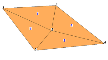
The following figure shows a 3D UGrid with three layers in oblique view.

The next two figures show the numbering of the points and cells on the top of the 3D UGrid, and on the 2D UGrid that would get generated by the tool if the "Top" option is selected. Notice the 2D UGrid numbering happens to match exactly with that of the 3D UGrid because the top points and cells start at one and there are no gaps in the numbering.

Example 1: 3D UGrid top numbering
Example 1: 2D UGrid from selecting "Top"


The next two figures show the numbering of the points and cells on the bottom of the 3D UGrid, and on the 2D UGrid that would get generated by the tool if the "Bottom" option is selected. Notice the 2D UGrid numbering differs from the bottom of the 3D UGrid but the order for both points and cells is the same.
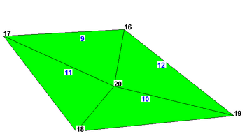
Example 1: 3D UGrid bottom numbering

Example 1: 2D UGrid from selecting "Bottom"


3D UGrid from Rasters
The 3D UGrid from Rasters tool is used to create a 3D UGrid from multiple rasters and a 2D UGrid by extruding the 2D UGrid and creating layers inbetween the rasters using the horizons approach. The resulting UGrid will be "stacked", meaning, there is no vertical sub-discretization of layers and the horizontal discretization of all layers is the same. Thus, no layers will pinch out, but layers may have zero thickness.
Input parameters
- 2D UGrid – The input 2D UGrid that will be used.
- Rasters – A table of rasters and their properties.
- Horizon – The horizon number. Horizons are automatically numbered consecutively in the order that the strata are “deposited” (from the bottom up).
- Fill – If checked, the raster will be used in the interpolation process for the associated UGrid point sheet (the points between cell layers) and one or more layers will be created below the raster.
- Clip – If checked, all rasters below (with a smaller horizon number) will not be permitted to go above the raster.
- Sublayers – Number of layers to create between the raster and the next raster below that has Fill checked. The default is 1.
- Proportions – Sublayer proportions as a space delimited list of integers, size of Sublayers, where 1 is the base thickness. For example "1 1 2" indicates three sublayers with the first two being the same thickness and the third being twice as thick as the first. If blank, sublayers (if any) will be evenly proportioned.
- Target location – Whether to calculate elevations at the UGrid cell tops and bottoms or at the points. For MODFLOW models, "Cell tops and bottoms" is appropriate; for HydroGeoSphere, "Points".
- Minimum layer thickness – The minimum thickness every layer must have. If necessary, points are moved down to satisfy this criteria, except for the top sheet of points.
Output parameters
- 3D UGrid name – Name of the 3D UGrid that will be created. If left blank, a default name is used.
Current location in Toolbox
Unstructured Grids/3D UGrid from Rasters
Examples
The following figure shows a slice through raster surfaces that have been indexed with horizon IDs.
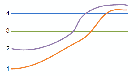 Raster surfaces.

Example 1
Below we see the resulting stratigraphy if the Clip field is off for each raster.
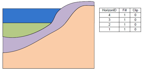 Stratigraphy with the Clip field turned off.

Example 2
This example shows how the stratigraphy changes when the Clip field is turned on for the top raster.
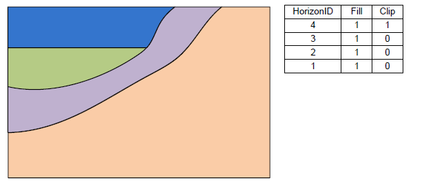 Stratigraphy with the Clip field on for horizon 4.

Example 3
This example shows how the stratigraphy changes when the Clip field is turned on for the raster with horizon 3.
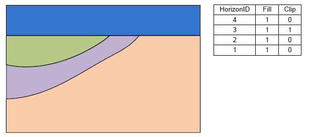 Stratigraphy with the Clip field on for horizon 3.

Example 4
The final example shows a case where the Fill field is off and the Clip field is on for the raster with horizon 3.
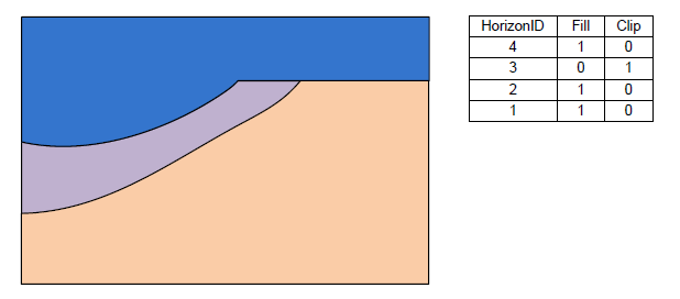 Stratigraphy with the Fill-off and Clip-on for horizon 3.

Related Tools
Export Curvilinear Grid
The Export Curvilinear Grid tool is used to create a curvilinear (boundary fitted) grid file (or files) for a curvilinear compatible mesh, scatter set or UGrid that is loaded into SMS. This can make use of user provided I,J index data sets if they exist. It also supports the option to compute I,J data indices. In this case, the orientation of the first cell in the surface will define the orientation of the I,J axes of the grid.
For EFDC grid files it may also use provided cell based datasets to populate the additional properties of the grid. These can include:
- Depth
- Z Roughness
- Vegetation type
- Wind shelter
Input Parameters
The format of the data file will be in either CH3D (also referred to as GSMB) or EFDC (also referred to as LTFATE). The input parameters include:
- Generate cell i-j datasets toggle.
- Cell i-coordinate dataset (optional) – Select the cell based dataset that defines the I index of each cell. This is required if the toggle to generate I-J is not selected.
- Cell j-coordinate dataset (optional) – Select the cell based dataset that defines the J index of each cell. This is required if the toggle to generate I-J is not selected.
Datasets that are available if the format is EFDC:
- Depth dataset (optional) – Select the cell based dataset to define the depth of each cell.
- Z Roughness dataset (optional) – Select the cell based to define the roughness of each cell.
- Vegetation type dataset (optional) – Select the cell based to define the vegetation type of each cell.
- Wind shelter dataset (optional) – Select the cell based to define the wind shelter value of each cell.
Output Parameters
The path to where files will be saved defaults to the project directory if one is defined in the instance of SMS. The path can be cut/paste from a file browser in windows to this edit field.
- CH3D grid file name defaults to "grid.inp".
- EFDC dxdy file name defaults to "dxdy.inp".
- EFDC lxly file name defaults to "lxly.inp".
- EFDC cell file name defaults to "cell.inp".
Current location in toolbox
This tool is currently located in Unstructured Grids/Export Curvilinear Grid.
Notes
The file formats for the CH3D and EFDC grids are defined in the Import Curvilinear Tool documentation. The cell.inp file for EFDC is not used for importing since it does not include any unique information for the definition of the grid. This file includes an ASCII map of the cell types in the grid.
Export UGrid
The Export UGrid tool exports the grid to a file; the file format is chosen as part of the tool inputs.
Input parameters
- UGrid – Select the grid in the project that will be exported
- File type – Select the desired output format.
- "Ascii XMC" – Aquaveo format for a UGrid which supports both structured and unstructured grids.
- "Binary XMC" – Aquaveo format for a UGrid.
- "Ascii STL" – Stereolithography file. This file contains the UGrid points and triangles. The UGrid must only have triangle cells to export this type of file.
- "Binary STL" – Stereolithography file.
- "OBJ" – OBJ geometry definition file. This file contains the UGrid points and triangles. The UGrid must only have triangle cells to export this type of file.
Output parameters
- Output file – This field will list the file directory for the exported grid file. Clicking the Save As... button will open a Save File dialog where the directory and file name can be set for the grid export.
Current Location in toolbox
Unstructured Grids/Export UGrid
Extract Subgrid
The Extract Subgrid tool is used to create a mesh that is a subset of another mesh or UGrid. When using the tool, an existing mesh or UGrid is required along with a map coverage containing a polygon that defines the subgrid domain.
A subgrid is often used to make edits to a portion of a grid that is too large to edit conveniently. If this is the case, when the edits are finished, the subgrid can be merged with the original grid.
Input parameters
- Grid – Select the base 2D mesh or UGrid in the project from which the subgrid will be extracted.
- Subgrid boundary coverage – Select a coverage in the project that contains a polygon which defines the boundaries of the subgrid domain.
Output parameters
- Grid name – Name of the 2D mesh that will be created.
Current location in Toolbox
Unstructured Grids/Edit Subgrid
Extrude UGrid
The Extrude UGrid tool converts a 2D UGrid into a 3D UGrid.
Input Parameters
- Input grid – Select a 2D UGrid to convert to a 3D UGrid.
- Number of layers – Enter the number of layers the new 3D UGrid will have.
- Layer n thickness – For each layer, enter the layer thickness. This value will be in the units set in the project projection.
Output Parameters
- Output grid – Name of the output grid.
Current Location in Toolbox
Unstructured Grids/Extrude UGrid
Fill Holes in UGrid
The Fill Holes in UGrid fills all voids in a given mesh with new mesh elements. The output is a mesh that can be converted back into a UGrid if needed. This tool also works on meshes.
Input Parameters
- 2D UGrid – Select a 2D UGrid that needs holes filled.
Output Parameters
- New Mesh Name – Enter the name that the output mesh should have.
Current Location in Toolbox
Unstructured Grids/Fill Holes in UGrid
Import Curvilinear Grid
The Import Curvilinear Grid tool is used to load an existing curvilinear (boundary fitted) grid into SMS as a UGrid object. This will also create cell based datasets defining the I, J index of each cell in the UGrid. Depending on the selected format and the specific data file(s).
For EFDC grid files it may also create additional cell based datasets for the UGrid that is loaded. These can include:
- Depth
- Z Roughness
- Vegetation type
- Wind shelter
Input parameters
- Format of the data file – Select the file format for the UGrid that will be imported.
- "CH3D" – Will import a CH3D file.
- "EFDC" – Will import a EFDC file.
- CH3D formatted grid file – Clicking the Select File button will open a Select File dialog where the CH3D file can be selected.
- EFDC formatted dxdy.inp file – Clicking the Select File button will open a Select File dialog where the dxyy.inp EFDC file can be selected.
- EFDC formatted lxly.inp file – Clicking the Select File button will open a Select File dialog where the lxly.inp EFDC file can be selected.
Output parameters
- Output UGrid name – Enter the name of the imported UGrid.
Current location in the toolbox
Unstructured Grids/Import Curvilinear Grid
CH3D Format
Format of the CH3D file (grid.inp). This file includes a 2 line header and a line for every corner point in a rectangular grid This includes inactive regions. The locations are ordered in a row major order. SMS will export 5 columns of data including (X, Y, Z, I, J). The (I, J) columns are not used in the import process. They are implied. The first line is a name to assign to the grid.
The second line defines the size of the grid based on cell corners. The number of cells in each direction is a maximum of the number of corners minus 1. Cell corners that do not correspond to an active cell in the grid is assigned a coordinate location of (9.0x10¹⁸, 9.0x10¹⁸, 9.0x10¹⁸).
Because this file format does not include cell based information, a single row or column of inactive cells is not supported. The corners of these cells are defined by the active neighbor, so the cell is assumed to exist. File organization:
    Grid_name
    num_rows_of_pts  num_cols_of_pts
    x y z 1 1
    x y z 2 1
    .
    .
    .
    x y z num_rows 1
    x y z 1 2
    x y z 2 2
    .
    .
    .
    x y z num_rows 2
    .
    .
    .
    x y z 1 num
Format of the EFDC files (dxdy.inp, lxly.inp). This format includes two files that work together to define the grid. The "dxdy.inp" files includes a 4 line comment header and a line for every active cell in the grid The header is metadata only and is not used in the import process. The last header line defines the values in each column for the data following. This includes:
- I J: the column and row index of the cell on this line.
- DX DY: the width and height of this cell.
- WATER DEPTH: the depth of the water in this cell.
- BOTTOM ELEV: the ground elevation value for this cell (cell based).
- ZROUGH: the roughness for this cell.
- VEG TYPE: the vegetation type for this cell.
The "lxly.inp" files also includes a 4 line comment header and a line for every active cell in the grid The header is metadata only and is not used in the import process. The last header line defines the values in each column for the data following. This includes:
- I J: the column and row index of the cell on this line.
- X Y: the location of the cell center of this cell.
- CUE CVE CUN CVN: the orientation of this cell (rotation values)
- WIND SHELTER: a wind shelter data value for this cell.
This format defines a nonconformal grid. Neighboring cells don't explicitly define the same corner points. When SMS loads this grid, the corner locations are merged to create a conformal grid. For this reason, when a grid is loaded and then rewritten, the detail definition may not be identical.
Import UGrid Points
The Import UGrid Points tool is used to import locations and datasets. The CSV file must contain coordinates for the points and, optionally, the file may contain datasets associated with the points.
The first line of the CSV file must be a header line with the coordinate columns of x, y, and z (optional). These columns must be named x, y, z. An error will be encountered if these columns do not exist.
Other columns may exist in the file for datasets. The dataset name is specified in the first line of the file. If the column does not have a name then the column will be skipped.
Transient data may also be imported using this tool. Transient datasets comprise multiple columns in the file with the same column name and with time specified on the second line of the file in the associated dataset column. There may not be any value specified on the second line of the file for the x, y coordinates. The time values may be relative times: 0.0, 2.5, 10.0, etc. Additionally, the time values may be specified as date times. The date format should be in the form of YEAR-MONTH-DAY HH:MM:SS.SS.
Multiple example files are shown below.
Input parameters
- CSV file with point coordinates and datasets – Shows the file name for the CSV file containing the coordinates and datasets. Clicking the Select File button will open a Select File browser dialog to select the CSV file.
- No data value – When the “No data value” is encountered in the csv file in one of the datasets XMS marks the value as “NULL” or “no data”. These values are not contoured or used in interpolation in XMS.
- Time unit – The time unit for transient datasets where the time is specified as a floating point number (in contrast to a date time).
- Coordinate system project file (*.prj) – Shows the file name for the projection associated with the coordinates of the points in the file. Clicking the Select File button will open a Select File browser dialog to select the PRJ file.
Current location in Toolbox
Unstructured Grids/Import UGrid Points
Example files
Example 1
id,y,x,c
1,15459458,2685809,6.4
2,15459506,2685824,9.7
3,15459524,2685850,8
This is a simple csv file. Notice the “x” and “y” columns; these are required. Note that “z” is not required. Also, notice that the order of x and y does not matter.
The other 2 columns: “id”, “c”. The will be imported as datasets.
Example 2
y	x	z	TDS	TDS	conc
			0	1
-16	-75	8.5	59.04	9.24	1.9
32	-60	9.8	90.2	71	4.8
50	-34	0.7	67.2	98.4	9.5
This example shows a file with “x”, ”y”, and “z” columns. Notice that there are no values on the second line of the file for x, y, and z. This indicates that times are being specified for the datasets in the file.
The other 2 columns: “TDS” and “conc”. The will be imported as datasets. TDS will be a transient dataset with times of 0.0 and 1.0. The user will have to specify the units of the times in the tool. The conc dataset will be imported without multiple time steps.
Example 3
y	x	c2	c2	c2
		2011-02-01	2012-02-01	2013-02-01
-16	-75	59.04	43.64	9.24
32	-60	90.2	44.16	71
50	-34	67.2	0	98.4
This is a csv file with a transient dataset with the time specified as dates.
Example 4
y	X	c2	c2	c2
		2011-02-01 15:30:22.1	2012-02-01	2013-02-01 6:45:15
-16	-75	59.04	43.64	9.24
32	-60	90.2	44.16	71
50	-34	67.2	0	98.4
This is a csv file with a transient dataset with the time specified as dates and times.
Map Activity to UGrid
This tool builds a unstructured grid (UGrid) using an existing geometry and an activity coverage. The resulting UGrid will not include areas designated as inactive in the activity coverage. The tool has the following options:
Input Parameters
- Input grid– Select the geometry that will define the values for the new UGrid.
- Activity coverage – Select the coverage that will define the activity for the new UGrid.
Output Paramters
- Name of the output ugrid – Enter the name for the new activity UGrid.
Current Location in Toolbox
Unstructured Grids/Map Activity to UGrid
Merge 2D UGrids
The Merge 2D UGrids tool merges two 2D geometries. These can be 2D meshes, 2D Grids, UGrids, or scatter sets. The geometries can overlap or not. In areas of overlap, the tool honors the primary grid, deletes all elements from the secondary grid that overlap part of the primary grid plus a buffer around the primary grid. This prevents the transition zone from becoming so small that poorly shaped cells result. The tool builds transition triangle cells to fill the gap created in this process. The new geometry is created as a 2D Mesh in SMS; in GMS, the tool output is a 2D UGrid.
Limitations:
- This tool only works on 2 geometries at a time. If multiple geometries are to be merged, they must be merged incrementally.
- The Primary grid must have defined cells/elements. Any disjoint points on the primary grid will be removed.
This tool is designed to replace the functionality to merge meshes and scatter sets in SMS. This operation is faster, more generic, and because it is in the toolbox, will be accessible outside of the standard SMS framework.
Input parameters
- Primary grid – Select the grid that will act as the primary grid. If there are conflicts during the merge, this grid will receive priority to resolve the conflict.
- Secondary grid – Select the grid that will act as the secondary grid during the merge.
- Duplicate point tolerance – When points are compared as duplicates the distance between the points is calculated. If the distance is less than this tolerance then the points are considered duplicates. This is used for comparing points on the outer boundary of the primary grid with points in the secondary grid and trying to preserve cells in the secondary grid that are adjacent to cells in the primary grid. The default value is usually sufficient but if you find cells in the secondary grid are being deleted and you want to preserve those then try increasing the tolerance.
- Buffer distance option – Option for buffering the outer boundary of the primary grid during the merge operation.
- Default – The tool will use 0.01 times the minimum cell edge length as the buffer distance.
- Specified – The tool will use the user specified buffer distance.
- Buffer distance – specify the desired buffer distance. This is the width of the transition zone between the geomtries.
- Stitch non-overlapping grids with matching boundary points – Option for merging two grids that have matching boundary points and no overlapping features. This option should only be used if the user is positive that the grids satisfy this constraint. A grid with internal holes will result from using this option when the grids overlap. The tool will run significantly faster if this option is checked.
Output parameters
- Merged grid – Enter the name of the new merged UGrid.
Current Location in toolbox
Unstructured Grids/Merge 2D UGrids
Refine UGrid
The Refine UGrid tool creates a 2D UGrid that has been refined based on an existing 2D UGrid and one or more elevation rasters.
Input parameters
- Grid – Select the 2D UGrid that will be refined.
- Default constant value – Enter a value for the desired average cell size for the new UGrid. It is important to note that the tool will refine the entire grid. If the default value is too small then there may be a long computation time for the tool. Entering a value that is too large may cause an error.
- Error threshold – Enter a value to guide the acceptable threshold for error for the grid refinement.
- Maximum iterations – The tool will perform multiple iterations when refining the new UGrid. Enter the maximum number of iterations to perform. The tool will stop performing iterations once it has reached the maximum limit if it has not completed refinement before this value is reached.
- Raster 1 (highest priority) – The elevation raster that will be used for refinement. This raster will be given priority over any additional rasters being used.
- Raster n – Allows selecting an additional raster to use in refinement.
Output parameters
- Output UGrid name – Enter the name for the new refined UGrid.
Current Location in toolbox
Unstructured Grids/Refine UGrid
Refine UGrid by Error
The Refine UGrid by Error tool creates a 2D UGrid that has been refined based on an existing 2D UGrid and one or more elevation rasters.
Input parameters
- Grid – Select the 2D UGrid that will be refined.
- Error threshold – Enter a value to guide the acceptable threshold for error for the grid refinement.
- Maximum iterations – The tool will perform multiple iterations when refining the new UGrid. Enter the maximum number of iterations to perform. The tool will stop performing iterations once it has reached the maximum limit if it has not completed refinement before this value is reached.
- Raster 1 (highest priority) – The elevation raster that will be used for refinement. This raster will be given priority over any additional rasters being used.
- Raster n – Allows selecting an additional raster to use in refinement.
Output parameters
- Output UGrid name – Enter the name for the new refined UGrid.
Current Location in toolbox
Unstructured Grids/Refine UGrid by Error
Relax UGrid Points
The Relax UGrid Points' tool adjusts point locations attempting to improve the quality of connected triangle cells. Usually the overall quality of the grid will improve but not in all cases. Some examples are of the tool are shown below.
Input parameters
- UGrid – Select the grid in the project that will have its points relaxed.
- Relaxation method – Select the desired relaxation method.
- "Area" – This method calculates the new location of a particular point by finding the centroid and area of all surrounding triangles and then computing a new location that is the weighted average of the triangle centroids. The weights are determined by the triangle area divided by the total area of all triangles connected to the point.
- "Angle" – This method attempts to make all the angles connected to a point equal. The new location is calculated such that the difference between connected angles is minimized.
- "Spring" – This method uses a size function (desired edge length) and spring force equation to move a point to the location that best satisfies the size function.
- "Lloyd" – This method is similar to area relax but seeks to move the particular point to the centroid of the voronoi polygon. It is recommended to use the “Optimize triangulation” when using the Lloyd relaxation option.
- See Wikipedia Lloyd’s algorithm - Lloyd's algorithm
- Implemented with guidelines from “Efficient mesh optimization schemes base on Optimal Delaunay Triangulations” Chen, Holst 2011)
- Number of iterations – The number of iterations to perform with the relaxation method
- Convergence distance – Early termination of the tool will occur if the maximum distance any point moves during an iteration is less than the convergence distance.
- Locked points dataset – A dataset where any nonzero value indicates that the point/node is locked and will not have its location adjusted by the tool.
- Spring relax size dataset – A dataset indicating the desired edge size at each point/node in the grid. This dataset must be specified if the relaxation method is “Spring”.
- Optimize triangulation – Before each smoothing step the triangles are checked to ensure they meet the Delaunay criteria. Any triangles that are not Delaunay compliant will be adjusted to satisfy the Delaunay criteria.
Output parameters
- Relaxed output grid name – Name of the output grid produced by the tool.
Outline of the tool algorithm
A basic outline of the algorithm is as follows:
- Build a list of all triangles in the input grid
- If optimizing the triangulation
- Ensure triangles satisfy Delaunay criterion
- Compute the initial quality of all triangles
- Ensure that all boundary points are locked (they may not move)
- For each iteration
- Compute the new location of all points using the specified method
- Check if the new locations will create any invalid triangles
- If invalid triangles are created then calculate new locations that are half the distance to the previous new locations and check again for invalid triangles
- Check for convergence if the maximum distance moved by any point is less than the convergence distance
- If convergence is not met and optimizing triangulation, optimize the triangles
- Compute final triangle quality
- Create the output grid
Discussion
Which smoothing option should I use? The answer to this question almost always depends on the particular application. The following are guidelines to help answer that question.
- Area relaxation and Lloyd relaxation produce similar results. Lloyd relaxation will typically move the points further from their original locations than area. This may be desirable in some application.
- Angle relaxation often gives better results than area relaxation when there is considerable area difference between triangles connected at a given point.
- Spring relaxation makes the most sense to use when the grid/mesh has been developed using a size function for the domain. Additionally, the boundaries used to generate the grid/mesh should be consistent with the size function.
Examples
Example 1
This example shows a grid with a uniform boundary spacing (5.0) with distribution of points on the interior.
- In this example, all of the relaxation methods perform well. The overall final cell/element quality is extremely high and the grids would be satisfactory for numerical analysis.

Area relax results with 5 iterations
| Quality | Min | Median | Mean | Std. Dev. |
| Initial Rr | 0.286 | 0.903 | 0.843 | 0.161 |
| Final Rr | 0.853 | 0.991 | 0.982 | 0.023 |

Angle relax results with 5 iterations
| Quality | Min | Median | Mean | Std. Dev. |
| Initial Rr | 0.286 | 0.903 | 0.843 | 0.161 |
| Final Rr | 0.853 | 0.989 | 0.983 | 0.023 |

Spring relax results with 5 iterations and constant size function of 5.0
| Quality | Min | Median | Mean | Std. Dev. |
| Initial Rr | 0.286 | 0.903 | 0.843 | 0.161 |
| Final Rr | 0.853 | 0.988 | 0.981 | 0.025 |

Lloyd relax results with 5 iterations
| Quality | Min | Median | Mean | Std. Dev. |
| Initial Rr | 0.286 | 0.903 | 0.843 | 0.161 |
| Final Rr | 0.855 | 0.989 | 0.980 | 0.025 |

Example 2
This example shows a grid with a uniform boundary spacing (5.0) with dense distribution of points near the center of the grid.

Area relax results with 5 iterations
| Quality | Min | Median | Mean | Std. Dev. |
| Initial Rr | 0.392 | 0.853 | 0.812 | 0.155 |
| Final Rr | 0.538 | 0.904 | 0.872 | 0.110 |

Angle relax results with 5 iterations
| Quality | Min | Median | Mean | Std. Dev. |
| Initial Rr | 0.392 | 0.853 | 0.812 | 0.155 |
| Final Rr | 0.376 | 0.928 | 0.889 | 0.117 |

Spring relax results with 5 iterations.
- Size function computed from the initial point spacing.
- Notice that the minimum quality metric decreased; the cell with the worst quality has become even worse.
| Quality | Min | Median | Mean | Std. Dev. |
| Initial Rr | 0.392 | 0.853 | 0.812 | 0.155 |
| Final Rr | 0.358 | 0.935 | 0.881 | 0.136 |

Lloyd relax results with 5 iterations
| Quality | Min | Median | Mean | Std. Dev. |
| Initial Rr | 0.392 | 0.853 | 0.812 | 0.155 |
| Final Rr | 0.394 | 0.872 | 0.831 | 0.144 |

Lloyd relax results with 5 iterations and optimize triangulation turned on.
| Quality | Min | Median | Mean | Std. Dev. |
| Initial Rr | 0.392 | 0.853 | 0.812 | 0.155 |
| Final Rr | 0.582 | 0.939 | 0.915 | 0.082 |

Example 3
This example shows a grid with a non-uniform boundary spacing. Note the longer boundary edge of the cell within the red box in the image below.

Area relax results with 5 iterations.
- The overall quality of the grid improves slightly. However, notice that the minimum quality metric has decreased; the cell with the worst quality has become even worse.
| Quality | Min | Median | Mean | Std. Dev. |
| Initial Rr | 0.371 | 0.921 | 0.899 | 0.093 |
| Final Rr | 0.267 | 0.928 | 0.902 | 0.102 |

Angle relax results with 5 iterations
- Similar to area relax. The overall quality of the grid improves slightly. However, notice that the minimum quality metric has decreased; the cell with the worst quality has become even worse.
| Quality | Min | Median | Mean | Std. Dev. |
| Initial Rr | 0.371 | 0.921 | 0.899 | 0.093 |
| Final Rr | 0.264 | 0.924 | 0.901 | 0.103 |

Spring relax results with 5 iterations and a size function computed from the initial point spacing
- This is difficult problem for the spring relax to solve because of the constrained boundary. Ideally, the boundary would be consistent with an overall size function that would be applied during the meshing process.
| Quality | Min | Median | Mean | Std. Dev. |
| Initial Rr | 0.371 | 0.921 | 0.899 | 0.093 |
| Final Rr | 0.092 | 0.923 | 0.897 | 0.115 |

Lloyd relax results with 5 iterations and optimize triangulation turned on.
- Similar to area relax. The overall quality of the grid improves slightly. However, notice that the minimum quality metric has decreased; the cell with the worst quality has become even worse.
| Quality | Min | Median | Mean | Std. Dev. |
| Initial Rr | 0.371 | 0.921 | 0.899 | 0.093 |
| Final Rr | 0.239 | 0.947 | 0.920 | 0.101 |

Example 4
This example shows a grid with fairly uniform boundary spacing and an internal feature that will be preserved using the locked nodes feature. The locked nodes are shown with dark red symbols.

Area relax results with 5 iterations.
| Quality | Min | Median | Mean | Std. Dev. |
| Initial Rr | 0.122 | 0.792 | 0.736 | 0.201 |
| Final Rr | 0.544 | 0.899 | 0.878 | 0.093 |

Angle relax results with 5 iterations
| Quality | Min | Median | Mean | Std. Dev. |
| Initial Rr | 0.122 | 0.792 | 0.736 | 0.201 |
| Final Rr | 0.522 | 0.913 | 0.889 | 0.087 |

Spring relax results with 5 iterations and a size function computed from the initial point spacing
| Quality | Min | Median | Mean | Std. Dev. |
| Initial Rr | 0.122 | 0.792 | 0.736 | 0.201 |
| Final Rr | 0.500 | 0.909 | 0.883 | 0.096 |

Lloyd relax results with 5 iterations and optimize triangulation turned on.
| Quality | Min | Median | Mean | Std. Dev. |
| Initial Rr | 0.122 | 0.792 | 0.736 | 0.201 |
| Final Rr | 0.590 | 0.927 | 0.898 | 0.091 |

UGrid from Coverage
The UGrid from Coverage tool creates a 2D unstructured mesh, or UGrid, from the feature objects on a selected coverage.
Input Parameters
- Coverage – Select a map coverage in the project.
Output Parameters
- Name of the output mesh – Enter a name for the new UGrid.
Current Location in Toolbox
Unstructed Grids/UGrid from Coverage
UGrid from Surface
The UGrid from Surface tool creates a new UGrid with copies of all of the datasets on the input mesh, scatter set, or Cartesian grid.
Input parameters
- Input grid – Select the input mesh, scatter set, or Cartesian grid to convert to a UGrid.
Output parameters
- Output grid name – Enter the name of the new Ugrid. If left blank the tool will use the name of the input UGrid.
Current location in Toolbox
Unstructured Grids/UGrid from Surface
Voronoi UGrid from UGrid
The Voronoi UGrid from UGrid tool creates a Voronoi UGrid from an existing geometry (2D Mesh, Scatter Set, or UGrid). The tool uses the centroid of each triangle, element or cell of the input geometry as a node in the resulting Voronoi UGrid. The cells around the edge of the UGrid are created by adding a Voronoi node at the bisection of the boundary edge and connecting that node to the node at the triangle/element/cell centroid.
These meshes can be passed into HEC-RAS 2D for analysis.
Input parameters
- Input grid – Select the geometry that will be converted to a Voronoi UGrid.
Output parameters
- Output grid name – Enter the name for the new Voronoi UGrid. This will be a UGrid because scatter sets and meshes do not support polygonal cells.
Current Location in toolbox
Unstructured Grids/Voronoi UGrid from UGrid
Example


| [hide] SMS – Surface-water Modeling System | ||
|---|---|---|
| Modules: | 1D Grid • Cartesian Grid • Curvilinear Grid • GIS • Map • Mesh • Particle • Quadtree • Raster • Scatter • UGrid |  |
| General Models: | 3D Structure • FVCOM • Generic • PTM | |
| Coastal Models: | ADCIRC • BOUSS-2D • CGWAVE • CMS-Flow • CMS-Wave • GenCade • STWAVE • WAM | |
| Riverine/Estuarine Models: | AdH • HEC-RAS • HYDRO AS-2D • RMA2 • RMA4 • SRH-2D • TUFLOW • TUFLOW FV | |
| Aquaveo • SMS Tutorials • SMS Workflows | ||