GMS:MF6 CHD Package
| This contains information about functionality available starting at GMS version 10.5. The content may not apply to other versions. |
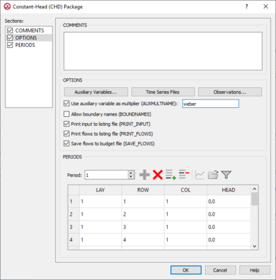
The Constant-Head (CHD) Package dialog is accessed by double-clicking on the CHD package under a MODFLOW 6 simulation in the Project Explorer. It contains the following sections and options:
- Sections list – A list of sections that can be turned on or off:
- Comments – Turn on to make the Comments section visible.
- Options – Turn on to make the Options section visible.
- Periods – Turn on to make the Periods section visible. This section is on by default.
- Comments section – Enter general alphanumeric comments. Comments entered here get written at the top of the file, preceded by a '#' symbol.
- Options section – Contains the following:
- Auxiliary Variables... – Click to bring up the Auxiliary Variables dialog.
- Time Series... – Click to bring up the Time Series Files dialog.
- Observations... – Click to bring up the Observation Files dialog.
- Use auxiliary variable as multiplier (AUXMULTNAME) – Name of auxiliary variable to be used as multiplier of CHD head value.
- Allow boundary names (BOUNDNAMES) – Turn on to allow boundary names to be included in the list of constant-head cells.
- Print input to listing file (PRINT_INPUT) – Turn on to write the list of constant-head information to the listing file immediately after it is read.
- Print flows to listing file (PRINT_FLOWS) – Turn on to write the list of constant-head flow rates to the listing file for every stress period time step in which "BUDGET PRINT" is specified in Output Control.
- Save flows to budget file (SAVE_FLOWS) – Turn on to write constant-head flow terms to the file specified with "BUDGET FILEOUT" in Output Control.
- Use with Water Mover (MVR) package (MOVER) – Turn on to allows this instance of the Constant-Head Package to be used with the Water Mover (MVR) Package.
- Periods section – Contains the following:
- Period drop-down – Use the Increment Up and Down
 buttons to select the desired period.
 - Define Period
 – If no period is defined, click to make the spreadsheet editable.
 - Delete Period
 – Click to delete the existing period.
 - Add Rows
 – Click to bring up the Add Stresses dialog.
 - Delete Rows
 – Click to bring up a dialog with three options:
- Delete from All Periods – Click to delete matching stresses from all periods.
- Delete from Just This Period – Click to delete matching stresses from just this period.
- Plot All Periods
 – Click to bring up the XY Series Editor dialog. Requires that a cell be selected in the table.
 - Open Time Series
 – Click to bring up the
 - Filter on Selected Cells
 – Click to turn on filtering on the selected cells.
- Table – Contains the following:
- LAY – Used to specify which layer is being applied.
- ROW – Used to specify which row is being applied.
- COL – Used to specify which column is being applied.
- HEAD – Represents the head at the boundary.
- Table – Contains the following:
- Period drop-down – Use the Increment Up and Down
Auxiliary Variables Dialog
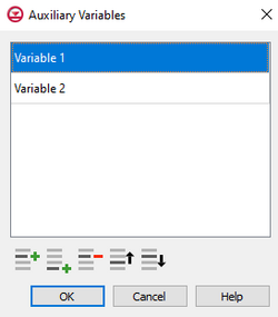
The Auxiliary Variables dialog is accessed by clicking Auxiliary Variables... in the Options section of many package dialogs. It is used to define an array of one or more auxiliary variable names. It contains the following sections and buttons:
- At the top is an unlabeled section listing all of the variables, one per line. Double-click on a variable name to rename it.
- Insert Row
 – Click to insert a row above the currently-selected row.
 - Add Row
 – Click to add a row below the currently-selected row.
 - Delete Row
 – Click to delete the selected row.
 - Move Up
 – Move the selected row up.
 - Move Down
 – Move the selected row down.
Note that each variable name must be unique. If two or more variables share a name, variables added since opening the dialog will not be saved.
Time Series Files Dialog
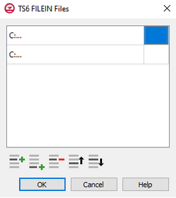
The Time Series Files dialog is accessed by clicking Time Series Files... in the Options section of many of the package dialogs. It is used to define an array of one or more time series files. It contains the following sections and buttons:
- At the top is an unlabeled section listing all of the time series files, one per line.
- Double-click on the first field to see the full file path and name.
- Click Edit... to open the time series file.
- Insert Row
 – Click to insert a row above the currently-selected row.
 - Add Row
 – Click to add a row below the currently-selected row.
 - Delete Row
 – Click to delete the selected row.
 - Move Up
 – Move the selected row up.
 - Move Down
 – Move the selected row down.
Observation Files Dialog
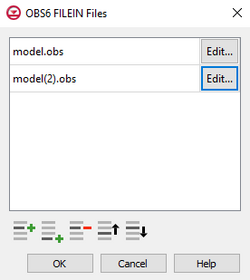
The Observation Files dialog is accessed by clicking Observations... in the Options section of many of the package dialogs. It is used to define an array of one or more observation files. It contains the following sections and buttons:
- At the top is an unlabeled section listing all of the observation files, one per line.
- Double-click on the first field to see the full file path and name.
- Click Edit... to open the Observations (OBS) Dialog.
- Insert Row
 – Click to insert a row above the currently-selected row.
 - Add Row
 – Click to add a row below the currently-selected row.
 - Delete Row
 – Click to delete the selected row.
 - Move Up
 – Move the selected row up.
 - Move Down
 – Move the selected row down.
Related Topics
GMS – Groundwater Modeling System | ||
|---|---|---|
| Modules: | 2D Grid • 2D Mesh • 2D Scatter Point • 3D Grid • 3D Mesh • 3D Scatter Point • Boreholes • GIS • Map • Solid • TINs • UGrids | |
| Models: | FEFLOW • FEMWATER • HydroGeoSphere • MODAEM • MODFLOW • MODPATH • mod-PATH3DU • MT3DMS • MT3D-USGS • PEST • PHT3D • RT3D • SEAM3D • SEAWAT • SEEP2D • T-PROGS • ZONEBUDGET | |
| Aquaveo | ||


