SMS:CMS-Flow Coverages
The CMS-Flow model makes use of the simulation based modeling approach. This requires defining coverages in the Map module to build the components for use in the CMS-Flow simulation.
Boundary Conditions
All numeric models require boundary condition data. In CMS-Flow, boundary conditions are defined on feature arcs in a boundary conditions coverage.
The Create Feature Arc can be used to click out boundary conditions for the model or arcs can be converted from other coverages or modules. Arcs can also be imported.
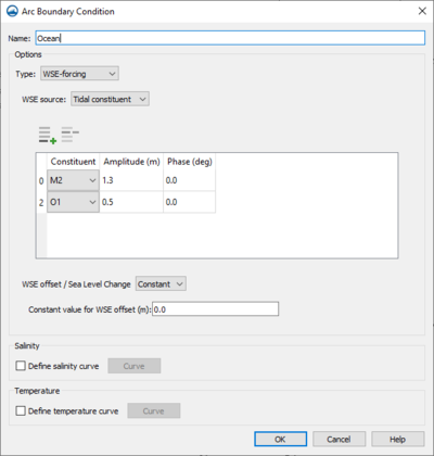
One the boundary condition arcs have been created, right-click on the arc with the Select Feature Arc tool and select the Assign Boundary Conditions command to bring up the Arc Boundary Condition dialog. This command is unique to the CMS-Flow Boundary Condition coverage and is only accessible by right-clicking on a selected arc.
Arc Boundary Conditions Dialog
This dialog has the following options for boundary condition parameters.
- Name – Assign a name to the boundary arc.
- Type – Has the following options:
- "Unassigned" – The default option.
- "Flow rate forcing" – Specifies an inflow rate (flow in cubic meters/second at each cell). This can be used to represent a river flowing into the domain.
- Flow Source – Specifies a time series of water fluxes as either a constant value or as a curve.
- "Constant" – Allows entering a Constant flow value for the flow rate in m^3/s per cell.
- "Curve" – Clicking the Curve button will bring up an XY Series Editor dialog where a time series of water fluxes can be entered.
- Specify inflow direction – Measured clockwise from North (degrees). Positive values are directed into the domain and negative values are leaving the domain. Will be perpendicular to the cell face if no value is set.
- Conveyance coefficient – Distributes the total volume flux across the boundary to estimate depth-averaged velocities. Default is equal to approximately 2/3 for uniform flow.
- Flow Source – Specifies a time series of water fluxes as either a constant value or as a curve.
- "WSE forcing" – Specifies the water surface elevation as a function of time for the cellstring. Options include specifying a single curve (water level -vs- time) and all the cells will have the same water level at the specified time and extracting individual curves for each cell either from a regional tidal database (ADCIRC database) or from a regional (larger) circulation model.
- WSE Source – The following WSE sources can be selected:
- "Constant" – Allows setting a Constant WSE value for the water surface elevation.
- "Curve" – Clicking the Curve button will bring up an XY Series Editor dialog where a time series for the water surface elevation can be entered.
- "Parent CMS-Flow" – This option will extract multiple time series curves from a larger CMS-Flow grid. Clicking the Select button will allow choosing the CMS-Flow data file.
- "Parent ADCIRC" – This option will extract multiple time series curves from an ADCIRC model. This type provides an option to Use Velocity from the ADCIRC model. The Parent grid (fort.14) file, ADCRIC Solution File Type, Parent solution file, and Parent Starting Time will all need to be selected.
- "Harmonic" – Option of forcing with a harmonic water surface elevation. With this option, the type of Speed, the Amplitude and the Phase can be entered in rows on the table.
- "Tidal Constituent" – Option of forcing with a tidal water surface elevation. With this option, the type of Constituent, the Amplitude and the Phase can be entered in rows on the table. Insert and delete rows to determine the constituents that will be used in the model run.
- "Tidal Database" – This option allows selecting a Tidal Database. Once the file has been selected, the Tidal Database Type needs to be specified as one of the following: "ADCIRC East Coast 2001", "ADCIRC West Coast 2003", "LeProvost 1994", "LeProvost 1995", or "LeProvost 2004". The number of Constituents is specified in the table by adding a row for each constituent included in the model run.
- WSE offset – An assumed spatially and temporally constant that may be used to correct the boundary water surface elevation for vertical data and sea level rise.
- WSE Source – The following WSE sources can be selected:
- Salinity – When this option is turned on, clicking the Curve button will bring up an XY Series Editor dialog where a time series of salinity values can be entered.
- Temperature – When this option is turned on, clicking the Curve button will bring up an XY Series Editor dialog where a time series of tempurature values can be entered.
Save Points
CMS-Flow includes save points which can be used to output calculations at specific locations.
Save points are created in the Save Points coverage using the Create Feature Point tool. When the coverage is linked to the CMS-Flow simulation data will be collected during the simulation model run.
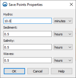
The coverage has two unique commands. The coverage right-click menu in the Project Explorer has a Properties command that will bring up the Save Points Properties dialog. Right-clicking on a point in the graphics window and selecting the Assign Save Points... command bring up the Assign Save Points dialog.
Save Points Properties Dialog
In the Save Points Properties dialog the output interval can be specified for data collected at each save point. The interval options can be specified for any of the following data types:
- Hydro
- Sediment
- Salinity
- Waves
All interval options can be specified in seconds, minutes, or hours.
Assign Save Points
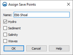
Each save point created in the coverage needs to be given parameters as to what type of data to collect during the simulation model run. Using the Select Feature Point tool, right-click on each save point and use the Assign Save Points... command. This will bring up the Assign Save Points dialog where the type of data to be gathered can be specified.
The dialog has the following options:
- Name – Each save point can be given a unique name. The given name will appear next to the point in the graphics window after being assigned.
- Hydro – Sets the save point to collect hydrologic data.
- Sediment – Sets the save point to collect sediment data.
- Salinity – Sets the save point to collect salinity data.
- Waves – Sets the save point to collect wave data.
Rubble Mound Jetties
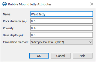
CMS-Flow allows creating polygons to represent rubble mound jetties. After a polygon has been created on the CMS-Flow Rubble Mound Jetties coverage, attributes can be assigned to the polygon by right-clicking on the polygon and selecting the Assign Rubble Mound Jetty command.
The Assign Rubble Mound Jetty dialog has for following options:
- Name – Each rubble mound can be given a unique name. The given name will appear next to the point in the graphics window after being assigned.
- Rock diameter – The average diameter of the jetty rock or riprap.
- Porosity – Enter the porosity value for the rubble mound jetty.
- Base depth – The starting depth of the rubble mound jetty.
- Calculation method – One of three different formulation equations can be used when including rubble mound jetties in the CMS-Flow simulation. They are as follows:
- "Sidropoulou et al. (2007)"
- "Kadlec and Knight (1996)"
- "Ward (1664)"
Related Topics
SMS – Surface-water Modeling System | ||
|---|---|---|
| Modules: | 1D Grid • Cartesian Grid • Curvilinear Grid • GIS • Map • Mesh • Particle • Quadtree • Raster • Scatter • UGrid |  |
| General Models: | 3D Structure • FVCOM • Generic • PTM | |
| Coastal Models: | ADCIRC • BOUSS-2D • CGWAVE • CMS-Flow • CMS-Wave • GenCade • STWAVE • WAM | |
| Riverine/Estuarine Models: | AdH • HEC-RAS • HYDRO AS-2D • RMA2 • RMA4 • SRH-2D • TUFLOW • TUFLOW FV | |
| Aquaveo • SMS Tutorials • SMS Workflows | ||


