GMS:Animations
One of the most powerful visualization tools in GMS is animation. Animations can be created with transient or steady state data. Furthermore, the view angle and zoom factor can be changed during the animation. Animations are saved in the Windows (*.avi) format. AVI files can be played back externally to GMS using a variety of applications and can be inserted into multi-media documents and applications.
A new animation can be created by selecting the Animate command from the Display menu.
The animation tools are included with all editions of GMS, including the community version.
Animation Options
There are multiple options available when creating an animation:
| Option | Type |
|---|---|
| Dataset | Transient |
| Particle Tracking | Transient |
| Cross-sections / Isosurfaces | Steady State |
| Moving View | N/A |
Transient vs. Steady State Animation
All of the options except Moving view are either considered Transient or Steady State. GMS does not allow use of a Transient option and a Steady State option at the same time. Moving view, however, can be used by itself or in conjunction with any combination of the other options.
The typical case for choosing to do a transient animation is when a project has a transient solution generated by a model. The transient animation could illustrate how vectors, contours, fringes or isosurfaces change at different solution times. A transient animation can also be used to show particle tracking over time, even with a steady state solution.
Steady state animation can only be performed using 3D grids or 3D meshes. A steady state animation can be used with a steady state dataset, or with one time step of a transient dataset. Two options are available for steady state animation: Cross-section / isosurface animation and flow trace animation.
Dataset Animation
Transient dataset animation can be used with any object with a transient dataset. As each frame is generated, a set of values corresponding to the current time is loaded into memory and the image is redrawn using the current display options. Thus, if the contours are turned on in the Display Options, the contours will vary from frame to frame according to the changes in the dataset.
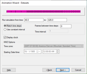
On the Datasets page of the dialog, the total number of frames generated in the animation can be defined in one of two ways:
- Matching time steps – A frame will be created for every time step in the project. Extra frames can be created between each time step if necessary using linear interpolation of the data values at the specified time steps. The desired number of frames between time steps can be set to the right of the Match time steps option.
- Use constant interval – Sets the interval at which animation frames are created. The number represents how many units to skip for each frame.
- Run simulation from time – Set the timeframe for the simulation based on the Reference time for the dataset being animated.
- Display clock – Sets a clock to display along with the animation.
- KMZ Options – Options related to creating a KMZ file. Only available when a KMZ file is being generated.
Particle Tracking Animation
Particle tracking can be animated to show how pathlines grow over time. Although it is considered a Transient option in the table above, this option can be used with a transient or a steady state solution. Only the forward tracking particle sets can be animated.
If Particle tracking is selected by itself, choose how many frames are wanted in the animation. GMS will then compute the time at which to generate each frame by dividing the total animation time evenly by the number of frames. The animation begins at the minimum start time of all forward tracking particle sets, and ends at the maximum travel time of all particles (in all forward tracking particle sets).
Cross-section / Isosurface Animation
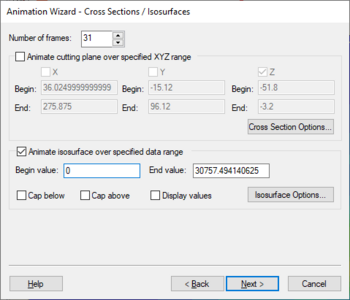
When the Cross-sections / Isosurfaces option is selected, a cutting plane and/or an isosurface can be animated. The Cross-sections / Isosurfaces page of the dialog specifies the parameters for the animation of these surfaces.
- Animate cutting plane over specified XYZ range – An x, y, and/or z cutting plane is incrementally moved through the mesh or grid from the specified beginning location to the ending location as each frame is generated. This generates an animation showing a moving cross section.
- Cross Section Options… – Opens a Cross Section Options dialog with all of the options available on the Cross Sections tab of the Display Options dialog. Adjusting the settings for cross sections here changes the settings in the Display Options dialog as well. It will immediately change the appearance of visible cross sections in the Graphics Window. This also affects the appearance of cross sections in the animation.
- Animate isosurface over specified data range – A single isovalue is incrementally varied between the specified beginning and ending values and a different isosurface is generated for each frame based on the value.
- Cap below – Displays an isosurface for all the values below the current values in the animation.
- Cap above – Displays an isosurface for all the values above the current values in the animation.
- Display values
- Isosurface Options – Opens the Isosurface Options dialog, which is the same dialog which can be accessed elsewhere in GMS. It has all settings previously set for isosurfaces in a project. Changing the settings here changes the settings for isosurfaces everywhere in the project.
Moving View
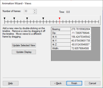
The Moving View option can be used by itself or in conjunction with any combination of the other options. This option can be used to change how to view the data as the animation proceeds. After selecting this option, set the desired distinct views using the tools on the Views page of the dialog. The timeline at the top of the Views page has a line for every frame. If there are many frames, each line may not be distinguishable from other lines.
Double-click on any one of the lines to create a new view. For a view that already exists, click on it to select it. A table appears with the data describing that view in the box on the right side of the dialog. The tools in the dialog allow for editing the view. This can be done in two ways:
- Update Selected View – Click this button to change the data in the table according to changes made in the display. To use this tool, first adjust the view in the Graphics Window. The Graphics Window can still be changed with the Animation Wizard open, so use the Static Tools or options from the Display | View menu to change the display in the Graphics Window, then click Update Selected View. The data in the table now reflects the adjusted display from the Graphics Window.
- Update Display – Click this button after changing the data in the dialog table. The display in the Graphics Window will update to reflect the data in the table.
Information on the meaning of Bearing and Dip is available on the GMS:Display Menu page under View Angle.
When the animation is generated, GMS will interpolate between the defined views to determine what the view should be at every frame.
CODEC
Starting in GMS 6.5 choose which codec to use to create an AVI movie. GMS will search the computer for all compatible codecs and they will be available in the pull down menu.
Animation Playback
Once a new animation has been generated, GMS launches the AVI player and plays the animation. The speed of playback can be adjusted using the Speed scroll bar. The maximum speed depends on the speed of the computer and the size of the image being animated. The smaller the image, the faster the maximum playback speed.
GMS – Groundwater Modeling System | ||
|---|---|---|
| Modules: | 2D Grid • 2D Mesh • 2D Scatter Point • 3D Grid • 3D Mesh • 3D Scatter Point • Boreholes • GIS • Map • Solid • TINs • UGrids | |
| Models: | FEFLOW • FEMWATER • HydroGeoSphere • MODAEM • MODFLOW • MODPATH • mod-PATH3DU • MT3DMS • MT3D-USGS • PEST • PHT3D • RT3D • SEAM3D • SEAWAT • SEEP2D • T-PROGS • ZONEBUDGET | |
| Aquaveo | ||


