GMS:Strike Dip Markov Chain: Difference between revisions
From XMS Wiki
Jump to navigationJump to search
No edit summary |
No edit summary |
||
| Line 1: | Line 1: | ||
{{T-PROGS Links}} | {{T-PROGS Links}} | ||
Once the vertical Markov chains have been defined, the user is then presented with the Strike (X) Markov Chains dialog. This dialog has the same general setup as the vertical dialog. | Once the vertical Markov chains have been defined, the user is then presented with the ''Strike (X) Markov Chains'' dialog. This dialog has the same general setup as the vertical dialog. | ||
==Strike (X) Markov Chains== | ==Strike (X) Markov Chains== | ||
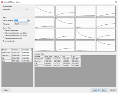
[[Image:markov_chains_x.png|thumb|400px|Strike/Dip Markov chain dialog.]] | [[Image:markov_chains_x.png|thumb|400px|''Strike/Dip Markov chain dialog''.]] | ||
There are three minor differences between this dialog and the vertical dialog. The first difference is in the [[GMS:Vertical Markov Chain|Markov Chains section]]. The option, Lens width ratios, replaces the Fit curves to a discrete lag option. The Fit curves to a discrete lag option is not applicable because horizontal measured transition probability curves do not exist due to lack of data in the horizontal direction. The Lens width ratios option is the default option and should be used in most cases. This option allows users to apply the transition data entered in the vertical direction to the horizontal direction. The proportion data are directly inherited from the vertical data. | There are three minor differences between this dialog and the vertical dialog. The first difference is in the [[GMS:Vertical Markov Chain|Markov Chains section]]. The option, Lens width ratios, replaces the Fit curves to a discrete lag option. The Fit curves to a discrete lag option is not applicable because horizontal measured transition probability curves do not exist due to lack of data in the horizontal direction. The Lens width ratios option is the default option and should be used in most cases. This option allows users to apply the transition data entered in the vertical direction to the horizontal direction. The proportion data are directly inherited from the vertical data. | ||
| Line 11: | Line 11: | ||
===Vertical->Lateral Data Conversion=== | ===Vertical->Lateral Data Conversion=== | ||
Typical site stratigraphic data is conducive to developing vertical spatial variability. However, rarely is the quantity of data adequate to develop an accurate model in the lateral directions. The combination of Walther’s Law and the transition probability approach allows for a logical method of developing lateral spatial variability from vertical spatial variability. Walther’s Law states that vertical successions of deposited facies represent the lateral succession of environments of deposition. Therefore, a logical method of generating a 3-D model of spatial variability would be first to develop a 1-D Markov chain in the [[GMS:Vertical Markov Chain|vertical direction]] based on site data, assuming there is such data. Second, using Walther’s Law and geologic knowledge, one can develop lateral, strike and dip, Markov chains of spatial variability. However, one issue that arises when applying vertical transition trends to lateral directions is how to cope with asymmetric vertical trends like fining upwards. For example, if in the vertical direction, sand tends to deposit on gravel as would be typical in a fluvial deposition, there will be a transition rate associated with the transition of sand->gravel and gravel->sand. The transition of gravel->sand will be greater than sand->gravel because of the fining upward trend. However, in the lateral direction, which of these transition rates should be applied? Although the trend of sand next to gravel remains in the lateral direction, the transition rates of sand->gravel and gravel->sand should be equivalent or symmetric as defined by | Typical site stratigraphic data is conducive to developing vertical spatial variability. However, rarely is the quantity of data adequate to develop an accurate model in the lateral directions. The combination of Walther’s Law and the transition probability approach allows for a logical method of developing lateral spatial variability from vertical spatial variability. Walther’s Law states that vertical successions of deposited facies represent the lateral succession of environments of deposition. Therefore, a logical method of generating a 3-D model of spatial variability would be first to develop a 1-D Markov chain in the [[GMS:Vertical Markov Chain|vertical direction]] based on site data, assuming there is such data. Second, using Walther’s Law and geologic knowledge, one can develop lateral, strike and dip, Markov chains of spatial variability. However, one issue that arises when applying vertical transition trends to lateral directions is how to cope with asymmetric vertical trends like fining upwards. For example, if in the vertical direction, sand tends to deposit on gravel as would be typical in a fluvial deposition, there will be a transition rate associated with the transition of "sand->gravel" and "gravel->sand". The transition of "gravel->sand" will be greater than "sand->gravel" because of the fining upward trend. However, in the lateral direction, which of these transition rates should be applied? Although the trend of sand next to gravel remains in the lateral direction, the transition rates of "sand->gravel" and "gravel->sand" should be equivalent or symmetric as defined by | ||
<!--[[Image:t-progs_eq4.png]]--> | <!--[[Image:t-progs_eq4.png]]--> | ||


