GMS:Vertical Markov Chain
| T-PROGS | |
|---|---|
| Links | |
| T-PROGS | |
| Strike Dip Markov Chain | |
| Vertical Markov Chain | |
| TSIM | |
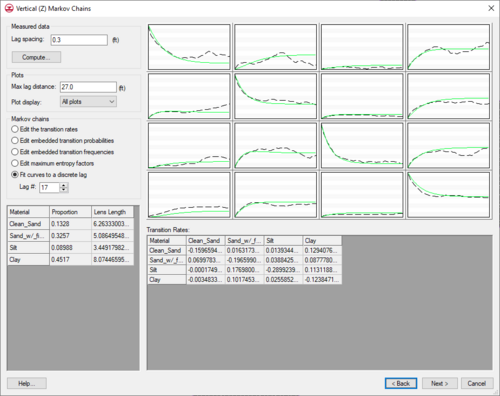
A dialog assists in defining the vertical Markov chains. This dialog is composed of three main sections:
- Plot section
- Markov Chains section
- Spreadsheet section
All three sections enable developing a 1-D Markov chain in the vertical direction.
Contents
Plot section
The plot section includes the array of curves, the Lag spacing edit field, the Compute button, and the Max lag distance for plots edit field. The number of plots in the array produced correlates to the number of materials used in the simulation. If N materials are used, an N by N array of plots will illustrate the transition probabilities for each material with respect to every other material. Every plot is labeled with a name and units and can be maximized with a command in the menu produced by right-clicking on the curve in question. The curves are automatically regenerated anytime a change is made in the other sections of the dialog.
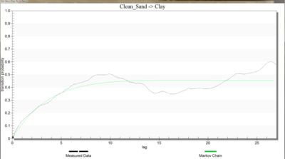
Each of the plots contains two curves depicting the transition probability. The dashed line represents the transition probability measured from the borehole data by the GAMEAS utility. In general, this curve represents the transition probability from material j to material k. The transition probability tjk(h) is defined by:
where x is a spatial location, h is the lag (separation vector), and j,k denote materials. The lag is defined by the Lag spacing item in the upper left corner of the Vertical (Z) Markov Chains dialog. The curve shown with the solid line is called a “Markov Chain”. The Markov Chains are used to formulate the equations used by T-PROGS to generate the multiple material sets during the simulation stage. The objective of this stage of the analysis is to fit the Markov Chain curves as accurately as possible to the measured transition probability curves. This process is similar to fitting a model variogram to an experimental variogram in a kriging exercise. The transition rates are adjusted to ensure a good fit between the Markov Chain model and the observed transition probability data.
Mathematically, a Markov Chain model applied to one-dimensional categorical data in a direction Φ assumes a matrix exponential form:
where Φ denotes a lag in the direction hΦ, and RΦ denotes a transition rate matrix
with entries rjk,Φ representing the rate of change from category j to category k (conditional to the presence of j) per unit length in the direction Φ. The transition rates are adjusted to ensure a good fit between the Markov Chain model and the observed transition probability data.
It should be noted that the self-transitional curves on the diagonal start at a probability of 1.0 and decrease with distance and the off-diagonal curves start at zero probability and increase with distance. In both cases, the curves eventually flatten out at some distance. The probability corresponding to the flat part of the curve represents the mean proportion of the material. All curves on a particular column should flatten out to the same proportion. The proportions are displayed in the lower left corner of the dialog. The point where a tangent line from the early part of the curves on the diagonal intersects the horizontal (lag distance) axis on each curve represents the mean lens length for the material. The mean lens lengths are shown just to the right of the mean proportions in the lower left part of the dialog. The slope at the beginning of each of the Markov Chains represents the transition rate. Together, the proportions, lens lengths, and transition rates define the Markov Chains.
Several methods are provided for fitting the Markov Chains to the measured transition probability curves. These methods are listed in the section of the dialog titled Markov Chains. By default, GMS automatically makes an attempt to fit the curves using the Edit maximum entropy factors option. In many cases, this fit is sufficiently accurate and we can proceed to the next step. However, it is often useful to explore the other options for fitting the curves.
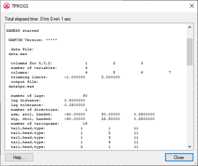
If boreholes exist in the model, the Compute... button becomes undimmed. When clicking the Compute... button, the parameter files required for running GAMEAS are generated and GAMEAS is executed.
GAMEAS
GAMEAS is an algorithm that processes borehole data and determines geologic characteristics such as material proportions and transition probability curves in a given direction. A separate window displays the details of the GAMEAS run, which allows monitoring the output from the GAMEAS simulation.
When GAMEAS completes a successful run, the results, including the material proportions and transition probability curves from the measured data, are read into the corresponding data fields in the Vertical Markov Chain dialog. Furthermore, the transition rates which correspond to the slope of the transition probability curves when the lag equals 0 are interpolated from the measured data curves. In addition to running GAMEAS, the code parses through the borehole data and calculates the embedded transition probabilities and frequencies. These values are stored in arrays that correspond to options #2 and #3 in the Markov Chains section of the dialog.
Lag
The Lag spacing determines how dense the curves are, and the Max lag distance for plots determines the range of the curves. The curves always range from 0 to the Max lag distance for plots horizontally, and they range from 0 to 1 vertically to honor probability constraints.
Markov chains section
There are five alternate methods of generating Markov chains in this section (area in the Vertical Markov Chain dialog). These methods are in a radio-button configuration to allow changing from one method to another. Each of these five methods will be described.
- Edit the transition rates
- Edit embedded transition probabilities
- Edit embedded transition frequencies
- Edit maximum entropy factors
- Fit curves to a discrete lag
- Edit the transition rates
Edit the transition rates
With this option one can directly edit the array of transition rates that are listed in the Transition Rates section. This option is useful after selecting the Compute button and running GAMEAS because slopes can be inferred from the measured data curves. GAMEAS outputs transition probability curves. Transition rates used in this option correspond to the slope of the transition probability curve at a lag = 0. When reading the output from GAMEAS, the transition probability rates are interpolated as:
where r1, r2, and r3 are the slopes defined by a straight line from the origin out to lag1, lag2, and lag3 respectively. As the lag approaches zero, more weight should be given to the corresponding slope. Hence, a weight of 0.57, 0.29, and 0.14 were assigned to r1, r2, and r3 respectively. Once the slopes are computed for each entry in the matrix, the mean lengths for each category are computed by:
Regardless of which Markov Chain option is selected, the background row and column, Sand_w/_fines, is dimmed because the values in this row and column are automatically computed from the remaining entries by probability constraints of the background material. In addition, with this option selected, the Lens Length column is also dimmed because the lens lengths are automatically computed and updated from the diagonal terms in the Transition Rates spreadsheet. The diagonal terms of the Transition Rates spreadsheet must be negative to obey probability rules. With this data, this method produces an accurate fit between the measured (green) and the Markov chain (blue) curves at small lag spaces.
Edit the embedded transition probabilities
This is a more intuitive method of generating Markov chains and is conducive to sites with and without data. It is conducive to sites with data because the embedded transition probabilities can be determined from the borehole data. When a simulation is initialized, if borehole data exist default embedded transition probabilities are computed from the borehole data. If borehole data do not exist, the embedded transition probabilities can be estimated with some basic geologic knowledge including the average mean lengths of each material for each direction and depositional trends.
With this option selected, the diagonal terms are dimmed because these values are derived from the values entered in the Lens Length column. Adjusting the proportions, lens lengths, or the off-diagonal terms in the Transition Rates spreadsheet alters the curves.
With this option, the spreadsheet in the lower right of the dialog represents the probability that the row material will transition to the column material moving vertically upwards in the +Z direction.
Edit the embedded transition frequencies
This option is similar to option #2, except embedded transition frequencies populate the off-diagonal terms of the Transition Rates spreadsheet. Embedded transition frequencies are also computed from borehole data when a simulation is initialized if borehole data exist. Once again, this is an intuitive framework with geologic knowledge including average mean lengths and depositional trends.
Edit maximum entropy factors
While this option can be used with borehole data, it is ideally suited for cases without borehole data. With this option, the user edits the proportions for all but the background material and the mean lens lengths for all materials. The lens lengths are used to populate the diagonal terms of the Transition Rates spreadsheet, and the maximum entropy factors fill the off-diagonal terms of the spreadsheet. The maximum entropy factors represent the ratio of the transition rate to the maximum entropy transition rate. A maximum entropy factor of 1.0 represents maximum disorder in depositional tendencies. A rate greater than 1.0 indicates that the two categories tend to occur next to each other. A factor less than unity would infer the opposite. This is an intuitive method of generating Markov chains and is conducive to all types of sites. This method enables logical incorporation of anisotropy into the model with the maximum entropy factors.
Fit curves to a discrete lag
This option is only undimmed if a transition probability curve from measured data exists in memory. When this option is selected, the Lag # edit field is undimmed to allow entering the discrete lag the curves will be fit to.
This option produces Markov chains that are computed from the measured transition rates produced by GAMEAS. GAMEAS computes a set of transition probabilities at each specified lag. This option computes an array of transition rates from the slope of the curves generated by GAMEAS (green). The transition rates correlate to the shape of the curve from the origin to the specified lag number in the Lag # edit field. Therefore, the cells of all the spreadsheets in the dialog are dimmed because the values are inherited from the measured curves (green). The values in the spreadsheets change depending on the lag # entered. By adjusting the lag interval, an excellent fit can often be obtained.
Spreadsheet section
This section includes two separate spreadsheets: Transition Rates and Proportions & Mean Lengths spreadsheets. The Transition Rates spreadsheet contains the rate entries that correspond to the selected option in the Markov Chains section. The Proportions column holds the proportions for each material. The Mean Lengths column contains the average mean length in the vertical direction for each material. The data in these spreadsheets define the Markov chains.
Notes
- ^ Carle, Steven F. (1999), T-PROGS: Transition Probability Geostatistical Software. Version 2.1, Davis, California, p. 6, http://gmsdocs.aquaveo.com/t-progs.pdf
| [hide]GMS – Groundwater Modeling System | ||
|---|---|---|
| Modules: | 2D Grid • 2D Mesh • 2D Scatter Point • 3D Grid • 3D Mesh • 3D Scatter Point • Boreholes • GIS • Map • Solid • TINs • UGrids | |
| Models: | FEFLOW • FEMWATER • HydroGeoSphere • MODAEM • MODFLOW • MODPATH • mod-PATH3DU • MT3DMS • MT3D-USGS • PEST • PHT3D • RT3D • SEAM3D • SEAWAT • SEEP2D • T-PROGS • ZONEBUDGET | |
| Aquaveo | ||


