GMS:Vertical Markov Chain: Difference between revisions
From XMS Wiki
Jump to navigationJump to search
(→Notes) |
|||
| Line 12: | Line 12: | ||
==Plot section== | ==Plot section== | ||
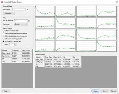
The plot section includes the array of curves, the Lag spacing edit field, the Compute button, and the Max lag distance for plots edit field. The number of plots in the array produced correlates to the number of materials used in the simulation. If N materials are used, an N by N array of plots will illustrate the transition probabilities for each material with respect to every other material. Every plot is labeled with a name and units and can be maximized with a command in the menu produced by right-clicking on the curve in question. The curves are automatically regenerated anytime a change is made in the other sections of the dialog. | The plot section includes the array of curves, the ''Lag spacing'' edit field, the '''Compute''' button, and the ''Max lag distance for plots'' edit field. The number of plots in the array produced correlates to the number of materials used in the simulation. If N materials are used, an N by N array of plots will illustrate the transition probabilities for each material with respect to every other material. Every plot is labeled with a name and units and can be maximized with a command in the menu produced by right-clicking on the curve in question. The curves are automatically regenerated anytime a change is made in the other sections of the dialog. | ||
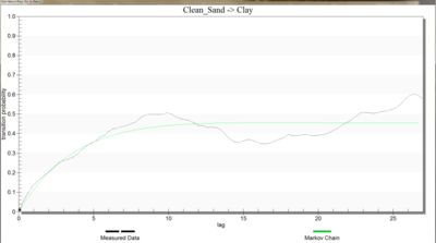
[[Image:markov_chain_plot.png|thumb|400px|Transition probability plot.]] | [[Image:markov_chain_plot.png|thumb|400px|Transition probability plot.]] | ||
Each of the plots contains two curves depicting the transition probability. The dashed line represents the transition probability measured from the borehole data by the GAMEAS utility. In general, this curve represents the transition probability from material j to material k. The transition probability t<sub>jk</sub>(h) is defined by: | Each of the plots contains two curves depicting the transition probability. The dashed line represents the transition probability measured from the borehole data by the GAMEAS utility. In general, this curve represents the transition probability from material j to material k. The transition probability ''t<sub>jk</sub>(h)'' is defined by: | ||
<!--[[Image:t-progs_eq1.png]] | <!--[[Image:t-progs_eq1.png]] | ||
| Line 30: | Line 30: | ||
|page=6 | |page=6 | ||
}}</ref></div> | }}</ref></div> | ||
where x is a spatial location, h is the lag (separation vector), and j,k denote materials. The lag is defined by the Lag spacing item in the upper left corner of the ''Vertical (Z) Markov Chains'' dialog. The curve shown with the solid line is called a “Markov Chain”. The Markov Chains are used to formulate the equations used by T-PROGS to generate the multiple material sets during the simulation stage. The objective of this stage of the analysis is to fit the Markov Chain curves as accurately as possible to the measured transition probability curves. This process is similar to fitting a model variogram to an experimental variogram in a kriging exercise. The transition rates are adjusted to ensure a good fit between the Markov Chain model and the observed transition probability data. | where ''x'' is a spatial location, ''h'' is the lag (separation vector), and ''j,k'' denote materials. The lag is defined by the Lag spacing item in the upper left corner of the ''Vertical (Z) Markov Chains'' dialog. The curve shown with the solid line is called a “Markov Chain”. The Markov Chains are used to formulate the equations used by T-PROGS to generate the multiple material sets during the simulation stage. The objective of this stage of the analysis is to fit the Markov Chain curves as accurately as possible to the measured transition probability curves. This process is similar to fitting a model variogram to an experimental variogram in a kriging exercise. The transition rates are adjusted to ensure a good fit between the Markov Chain model and the observed transition probability data. | ||
It should be noted that the self-transitional curves on the diagonal start at a probability of 1.0 and decrease with distance and the off-diagonal curves start at zero probability and increase with distance. In both cases, the curves eventually flatten out at some distance. The probability corresponding to the flat part of the curve represents the mean proportion of the material. All curves on a particular column should flatten out to the same proportion. The proportions are displayed in the lower left corner of the dialog. The point where a tangent line from the early part of the curves on the diagonal intersects the horizontal (lag distance) axis on each curve represents the mean lens length for the material. The mean lens lengths are shown just to the right of the mean proportions in the lower left part of the dialog. The slope at the beginning of each of the Markov Chains represents the transition rate. Together, the proportions, lens lengths, and transition rates define the Markov Chains. | It should be noted that the self-transitional curves on the diagonal start at a probability of 1.0 and decrease with distance and the off-diagonal curves start at zero probability and increase with distance. In both cases, the curves eventually flatten out at some distance. The probability corresponding to the flat part of the curve represents the mean proportion of the material. All curves on a particular column should flatten out to the same proportion. The proportions are displayed in the lower left corner of the dialog. The point where a tangent line from the early part of the curves on the diagonal intersects the horizontal (lag distance) axis on each curve represents the mean lens length for the material. The mean lens lengths are shown just to the right of the mean proportions in the lower left part of the dialog. The slope at the beginning of each of the Markov Chains represents the transition rate. Together, the proportions, lens lengths, and transition rates define the Markov Chains. | ||
| Line 42: | Line 42: | ||
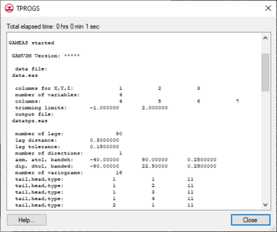
GAMEAS is an algorithm that processes borehole data and determines geologic characteristics such as material proportions and transition probability curves in a given direction. A separate window displays the details of the GAMEAS run, which allows the user to monitor the output from the GAMEAS simulation. | GAMEAS is an algorithm that processes borehole data and determines geologic characteristics such as material proportions and transition probability curves in a given direction. A separate window displays the details of the GAMEAS run, which allows the user to monitor the output from the GAMEAS simulation. | ||
When GAMEAS completes a successful run, the results, including the material proportions and transition probability curves from the measured data, are read into the corresponding data fields in the ''Vertical Markov Chain'' dialog. Furthermore, the transition rates which correspond to the slope of the transition probability curves when the lag equals 0 are interpolated from the measured data curves. In addition to running GAMEAS, the code parses through the borehole data and calculates the embedded transition probabilities and frequencies. These values are stored in arrays that correspond to options #2 and #3 in the Markov Chains section of the dialog. | When GAMEAS completes a successful run, the results, including the material proportions and transition probability curves from the measured data, are read into the corresponding data fields in the ''Vertical Markov Chain'' dialog. Furthermore, the transition rates which correspond to the slope of the transition probability curves when the lag equals 0 are interpolated from the measured data curves. In addition to running GAMEAS, the code parses through the borehole data and calculates the embedded transition probabilities and frequencies. These values are stored in arrays that correspond to options #2 and #3 in the ''Markov Chains'' section of the dialog. | ||
===Lag=== | ===Lag=== | ||
The Lag spacing determines how dense the curves are, and the Max lag distance for plots determines the range of the curves. The curves always range from 0 to the Max lag distance for plots horizontally, and they range from 0 to 1 vertically to honor probability constraints. | The ''Lag spacing'' determines how dense the curves are, and the Max lag distance for plots determines the range of the curves. The curves always range from 0 to the Max lag distance for plots horizontally, and they range from 0 to 1 vertically to honor probability constraints. | ||
==Markov chains section== | ==Markov chains section== | ||


