GMS:3D Interpolation Options: Difference between revisions
| Line 13: | Line 13: | ||
===Interpolation Methods=== | ===Interpolation Methods=== | ||
The following methods are supported for 3D interpolation in GMS: | The following [[GMS:Interpolation|methods]] are supported for 3D interpolation in GMS: | ||
*[[GMS:Inverse Distance Weighted|Inverse Distance Weighted Interpolation]] | *[[GMS:Inverse Distance Weighted|Inverse Distance Weighted Interpolation]] | ||
Revision as of 21:33, 30 December 2015
3D scatter point sets are used for interpolation to other data types such as grids and meshes. Interpolation is useful for such tasks as isosurface rendering or setting up input data for a model. Since no interpolation scheme is superior in all cases, several interpolation techniques are provided in GMS.
The basic approach to performing an interpolation is to select an appropriate interpolation scheme and interpolation parameters, and then interpolate to the desired object using one of the interpolation commands (to 3D Grid, to 3D Mesh, etc.) described below.
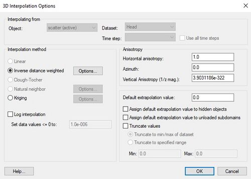
The interpolation options are selected using the 3D Interpolation Options dialog which is accessed through the Interpolation Options command in the Interpolation menu. Once a set of options is selected, those options are used for all subsequent interpolation commands. The options in the 3D Interpolation Options dialog are as follows:
Active Dataset
Interpolation is always performed using the active dataset of the active scatter point set. The active dataset is normally selected in the Project Explorer. The name of the current active dataset is listed at the top of the 3D Interpolation Options dialog.
If the active dataset is transient then more interpolation options are available. (see Steady State vs. Transient Interpolation)
Interpolation Methods
The following methods are supported for 3D interpolation in GMS:
Log interpolation is also supported.
Anisotropy
Sometimes the data associated with a scatter point set will have directional tendencies. The azimuth and horizontal anisotropy allow the user to take into account these tendencies.
Vertical Anisotropy
In 3D, vertical anisotropy is also available. In previous versions of GMS the user could enter a Z scale. Vertical anisotropy is 1 over the Z scale. This notation was changed to be consistent with Kriging.
Occasionally, scatter point sets are sampled along vertical traces. In such cases, the distances between scatter points along the vertical traces are an order of magnitude smaller than the distances between scatter points along the horizontal plane. For example, if the scatter point set was obtained from borehole data, the distance between scatter points may be a few centimeters, whereas the distance between boreholes may be several meters. This disparity in scaling causes clustering and can be a source of poor results in some interpolation methods.
The effects of clustering along vertical traces can be minimized using the vertical anisotropy option in the 3D Interpolation Options dialog. The Z coordinate of each of the scatter points is multiplied by 1 / the vertical anisotropy parameter prior to interpolation. Thus, if the vertical anisotropy parameter is less than 1.0, scatter points along the same vertical axis appear farther apart than they really are and scatter points in the same horizontal plane appear closer than they really are. As a result, points in the same horizontal plane are given a higher relative weight than points along the Z axis. This can result in improved accuracy, especially in cases where the horizontal correlation between scatter points is expected to be greater than the vertical correlation (which is typically the case in soils since soils are deposited in horizontal layers).
This option will assign the default extrapolation value to all cells that are hidden using the Hide command in the Display | Visibility menu option (see Display Menu).
Truncation
When interpolating a set of values, it is sometimes useful to limit the interpolated values to lie between a minimum and maximum value. For example, when interpolating contaminant concentrations, a negative value of concentration is meaningless. However, many interpolation schemes will produce negative values even if all of the scatter points have positive values. This occurs in areas where the trend in the data is toward a zero value. The interpolation may extend the trend beyond a zero value into the negative range. In such cases it is useful to limit the minimum interpolated value to zero. Interpolated values can be limited to a given range by selecting the Truncate values option in the 3D Interpolation Options dialog.
Related Topics
GMS – Groundwater Modeling System | ||
|---|---|---|
| Modules: | 2D Grid • 2D Mesh • 2D Scatter Point • 3D Grid • 3D Mesh • 3D Scatter Point • Boreholes • GIS • Map • Solid • TINs • UGrids | |
| Models: | FEFLOW • FEMWATER • HydroGeoSphere • MODAEM • MODFLOW • MODPATH • mod-PATH3DU • MT3DMS • MT3D-USGS • PEST • PHT3D • RT3D • SEAM3D • SEAWAT • SEEP2D • T-PROGS • ZONEBUDGET | |
| Aquaveo | ||
