SMS:Observation Coverage
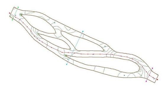
SMS contains what is called an observation coverage that is designed to help in model verification and calibration processes. Result verification is an important part of the computer modeling process. SMS includes a number of powerful tools, associated with an observation coverage, that allow users to verify simulation results with observed data. The two tools used for verification and calibration in an observation coverage are observation points and observation arcs. Observation points are used to verify the numerical analysis with measured field data such as water surface elevation or velocity data. They are also be used to see how computed values change with time at a particular location. Observation arcs are used to view the results at a cross section or along the river profile. These tools can be used with any of the SMS models.
Creating an Observation Coverage
To create a new observation coverage:
- Right-click the Map Data item in the Project Explorer
- Select New Coverage from the right-click menu
- Set the coverage type to Generic → Observation in the New Coverage Dialog
- Set the coverage name as desired
- Click OK to exit the dialog
Alternatively, an existing coverage can be changed to an observation coverage by right-clicking on the coverage in the Project Explorer and setting the type to Observation using the right-click menu.
Creating an Observation Point
Observation points are created at locations in the model where calibration data such as the velocity or water surface elevation has been measured in the field. Each observation point is used to compare the measured values with the values computed by the model at the point's x, y location. This comparison can assist the modeler in determining the accuracy of the numerical model results. If the numerical model results do not match the observed field data, model parameters such as manning's roughness may need to be modified to obtain more accurate results.
Creating an observation point is just like creating a feature point in any other coverage type. Select the Create Feature Point tool from the Dynamic Toolbar and click the location for the feature point.
Creating an Observation Arc
Observation arcs are created at cross sections in the model where calibration data such as the flowrate has been measured in the field. Observation arcs compute fluxes across the arc. Therefore, measurements for observation arcs are called Flux Measurements. Each obseration arc is used to compare the measured values with the values computed by the model across the vertical plane defined by the arc. This comparison can assist the modeler in determining the accuracy of the numerical model results. If the numerical model results do not match the observed field data, model parameters such as manning's roughness may need to be modified to obtain more accurate results.
Creating an observation arc is just like creating a feature arc in any other coverage type. Select the Create Feature Arc tool from the Dynamic Toolbar and click out your arc. Double-click to end the arc. In an observation coverage, profile arcs and cross section arcs may be useful to analyze a simulation's solution.
Setting Observation Object Attributes
Observation point and arc attributes are defined in the Observation Coverage dialog. See Observation Coverage dialog for a description of the Observation Coverage dialog.
Viewing Results
In addition to viewing the results of the solution data versus the observed data on the calibration targets, additional plots can be created using the Plot Wizard. See Plot Window for a description of the available plot types.
Calibration
Calibration is the process of modifying the input parameters to a model until the output from the model matches an observed set of data. SMS includes a suite of tools to assist in the process of calibrating a model. Both point and flux observations are supported. Most of the calibration tools can be used with any of the models in SMS.
Measurement types can be defined in SMS. They are defined in the map module and are associated with points and arcs in an observation coverage. Point observations represent locations in the field where some value has been observed. In most cases, the points will correspond to gauges or high water marks and the value will be the elevation of the water (the head) or a flow velocity (and possibly direction). Flux observations represent linear or areal objects such as streams gages where the flow rate has been measured or estimated. Both point and flow observations can be assigned a confidence interval or calibration target.
Once a set of observed point and flow values has been entered, each time a model solution is imported, SMS automatically interpolates the computed solution to the observation points. A calibration target representing the magnitude of the residual error is displayed next to each observation point and each flux object as shown below. The size of the target is based on the confidence interval or the standard deviation. In addition to the calibration targets next to the observation points, you can choose to display any of a number of statistical plots.
Calibration Target
If an observed value has been assigned to an observation point or if an observed flow has been assigned to an arc or polygon, the calibration error at each object can be plotted using a "calibration target". A set of calibration targets provides useful feedback on the magnitude, direction (high, low), and spatial distribution of the calibration error.
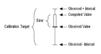
The components of a calibration target are illustrated in the following figure. The center of the target corresponds to the observed value. The top of the target corresponds to the observed value plus the interval and the bottom corresponds to the observed value minus the interval. The colored bar represents the error. If the bar lies entirely within the target, the color bar is drawn in green. If the bar is outside the target, but the error is less than 200%, the bar is drawn in yellow. If the error is greater than 200%, the bar is drawn in red. The display options related to calibration targets are specified in the Calibration Display Options dialog.
If the active time step is before the first observed time, or after the last observed time, the targets are drawn lighter.
Calibration Display Options
Calibration targets are drawn next to their corresponding map data (point, arc, polygon). The Feature Objects Display Options dialog contains a toggle labeled calibration targets. Below the toggle is a Scale edit field.
The target is drawn such that the height of the target is equal to twice the confidence interval (+ interval on top, - interval on bottom). The Scale edit field allows the user to change the general length and width of the targets independent of the range of the active dataset.
Observation Coverage Dialog
The Observation Objects dialog has two sections used to define the attributes of the points and arcs created in the observation coverage. To open the Observation Coverage dialog:
- Make the observation coverage active in the Project Explorer
- Select the Create Feature Point or Create Feature Arc tool from the Dynamic Toolbar
- Select a feature point or feature arc
- Select the menu command Feature Objects | Attributes or double-click in the previous step
Dialog Layout
The options in the dialog will differ slightly based on the feature object type currently being edited (arc or point). The feature object type is specified using the combo box in the upper right of the dialog.
In addition to a unique Name and Dataset(s), two other parameters are used to define the data represented by a measurement: Trans and Module. When analyzing data that varies through time, select the Trans toggle. The Module of a measurement refers to the SMS module where the computed data is stored. (The Module is set by default and normally does not need to be changed.)
Observation Point Attributes
When "points" is selected in the Feature object type combo box, the top section of the dialog is entitled Measurements and the bottom section is entitled Observation Points. The Measurements section is used to specify which datasets correspond with the observed data entered in the Observation Points section. The Measurements section is used to enter the observed data at each point. Each observation point is assigned the following attributes:
- Color – Color of the observation point.
- Observe – Turn the observation point on or off.
- Name – Name of the observation point.
- X – X-location of the point.
- Y – Y-location of the point.
- Observed Value – Value measured in the field corresponding to the active measurement.
- Interval – Allowable error (±) between the computed value and the observed value. Model verification is achieved when the error is within the interval (±) of the observed value.
- Angle – When a measurement for observation points is tied to a vector dataset (as is the case with a Velocity measurement) an angle needs to be specified. This angle is an azimuth angle with the top of the screen representing north when in plan view.
Observation Arc Attributes
If "arcs" is selected in the combo box, then the top spreadsheet had the name Flux Measurements and the bottom spreadsheet has the name of Observation Arcs.
To define an arc measurement, the Name must first be defined. In addition to a unique Name, a scalar and vector dataset must be assigned to it. Two other parameters are also used to define the data represented by a measurement: Trans and Module. When analyzing data that varies through time, select the Trans toggle. The Module of a measurement refers to the SMS module where the computed data is stored. (The Module is set by default and normally does not need to be changed.)
Each observation arc is assigned the following attributes:
- Color – Color of the observation arc.
- Observe – Turn the observation arc on or off.
- Name – Name of the observation arc.
- x-origin – X origin of the arc (used to modify the x-value used in plots).
- Observed Value – Value measured in the field corresponding to the active measurement.
- Interval – Allowable error (±) between the computed value and the observed value. Model verification is achieved when the error is within the interval (±) of the observed value.
Related Topics
SMS – Surface-water Modeling System | ||
|---|---|---|
| Modules: | 1D Grid • Cartesian Grid • Curvilinear Grid • GIS • Map • Mesh • Particle • Quadtree • Raster • Scatter • UGrid |  |
| General Models: | 3D Structure • FVCOM • Generic • PTM | |
| Coastal Models: | ADCIRC • BOUSS-2D • CGWAVE • CMS-Flow • CMS-Wave • GenCade • STWAVE • WAM | |
| Riverine/Estuarine Models: | AdH • HEC-RAS • HYDRO AS-2D • RMA2 • RMA4 • SRH-2D • TUFLOW • TUFLOW FV | |
| Aquaveo • SMS Tutorials • SMS Workflows | ||

