GMS:Pilot Points: Difference between revisions
From XMS Wiki
Jump to navigationJump to search
| (11 intermediate revisions by the same user not shown) | |||
| Line 1: | Line 1: | ||
{{Infobox Calibration}} | {{Infobox Calibration}} | ||
__TOC__ | |||
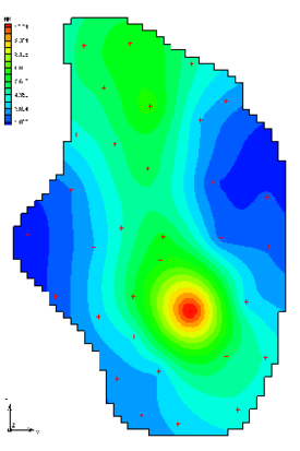
Pilot points can be thought of as a 2D scatter point set. Instead of creating a zone and having the inverse model estimate one value for the entire zone, the value of the parameter within the zone is interpolated from the pilot points. Then the inverse model estimates the values at the pilot points. The figure below shows a set of pilot points used to estimate horizontal hydraulic conductivity. Notice how the hydraulic conductivity now varies from cell to cell. When the inverse model runs, the values at the pilot points are adjusted and the “surface” defining the variation of K values is warped until the objective function is minimized. | Pilot points can be thought of as a 2D scatter point set. Instead of creating a zone and having the inverse model estimate one value for the entire zone, the value of the parameter within the zone is interpolated from the pilot points. Then the inverse model estimates the values at the pilot points. The figure below shows a set of pilot points used to estimate horizontal hydraulic conductivity. Notice how the hydraulic conductivity now varies from cell to cell. When the inverse model runs, the values at the pilot points are adjusted and the “surface” defining the variation of K values is warped until the objective function is minimized. | ||
PEST provides an additional option for the pilot point method called “regularization”. Regularization imposes an additional measure of “stiffness” to the parameter being interpolated via a “homogeneity” constraint. In the absence of any strong influence from the PEST objective function, this constraint causes values at pilot points to approximate the mean value of adjacent pilot points. This constraint makes the inversion process much more stable and makes it possible to violate one of the typical constraints associated with parameter estimation: namely, the requirement that the number of parameters must be less than the number of observations. With regularization, the number of parameters can greatly exceed the number of observations. As a result, complex hydraulic conductivity distributions can be defined, resulting in extremely low residual error. The pilot point method with regularization is an incredibly powerful feature of PEST. (For more on PEST see [[GMS:Automated Parameter Estimation|Automated Parameter Estimation]]) | PEST provides an additional option for the pilot point method called “regularization”. Regularization imposes an additional measure of “stiffness” to the parameter being interpolated via a “homogeneity” constraint. In the absence of any strong influence from the PEST objective function, this constraint causes values at pilot points to approximate the mean value of adjacent pilot points. This constraint makes the inversion process much more stable and makes it possible to violate one of the typical constraints associated with parameter estimation: namely, the requirement that the number of parameters must be less than the number of observations. With regularization, the number of parameters can greatly exceed the number of observations. As a result, complex hydraulic conductivity distributions can be defined, resulting in extremely low residual error. The pilot point method with regularization is an incredibly powerful feature of PEST. (For more on PEST see [[GMS:Automated Parameter Estimation|Automated Parameter Estimation]]) | ||
[[Image:pilot.png|thumb|none|275 px|Pilot points and resulting conductivity field]] | |||
==Interpolation Options== | |||
[[GMS:Kriging|Kriging]] and [[GMS:Inverse Distance Weighted|IDW]] are the only interpolation options supported with pilot points. The kriging option requires the establishment of a model variogram (by creating a nested structure). The nodal function options in the IDW method are not supported because those schemes compute gradients based on the dataset values at the surrounding points. With the pilot point method, the values at the points will change during the inversion process, thereby rendering the previously computed gradients inaccurate. | |||
[[GMS:Kriging|Kriging]] and [[GMS:Inverse Distance Weighted|IDW]] are the only interpolation options supported with pilot points. The kriging option requires the establishment of a model variogram (by creating a nested structure). The nodal function options in the IDW method are not supported because those schemes compute gradients based on the | |||
==Pilot Point Conditioning== | |||
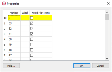
For pilot point interpolation of hydraulic conductivity, it is sometimes useful to include one or more measured K values with the pilot point set. These measured values could represent K values extracted from a field pump test. The ''Pilot Point Conditioning'' option is available to represent this scenario. One of the properties associated with scatter points is a ''Fixed pilot point'' toggle. | For pilot point interpolation of hydraulic conductivity, it is sometimes useful to include one or more measured K values with the pilot point set. These measured values could represent K values extracted from a field pump test. The ''Pilot Point Conditioning'' option is available to represent this scenario. To access this options: | ||
#Use the '''Select Scatter Point''' tool to select scatter points in the desired scatter set. | |||
#Double-click on the selected point, or right-click on the scatter points and select the '''Properties''' command. | |||
#The ''Properties'' dialog that appears will display all selected points. Unselected points will not be available. | |||
One of the properties associated with scatter points is a ''Fixed pilot point'' toggle. If this toggle is on and the corresponding scatter point set is used for pilot point interpolation, the K value assigned to the point is not allowed to vary during the parameter estimation process. | |||
[[Image:Pilot_Point_Cond. | [[Image:Pilot_Point_Cond.png|thumb|none|left|380px]] | ||
==Guidelines for Placement of Pilot Points== | |||
Note: The recommended maximum number of pilot points is about 200. | Note: The recommended maximum number of pilot points is about 200. | ||
# Place points between observations rather than on top of observations | # Place points between observations rather than on top of observations | ||
| Line 32: | Line 34: | ||
{{Navbox GMS}} | {{Navbox GMS}} | ||
[[Category:Parameters]] | [[Category:Parameters]] | ||
[[Category:GMS Dialogs|P]] | |||

