GMS:MODFLOW-USG Observations
MODFLOW-USG does not support an observation process as does MODFLOW 2000, 2005, NWT, ect. When using MODFLOW-USG in GMS a series of PEST utilities are run to calculate the model computed values at observations. The inputs to these utilities are managed in the MODFLOW-USG Observation dialog. This dialog contains information for head observations as well as flow observations. The head and flow observations can be steady state or transient depending on the type of MODFLOW-USG simulation.
Generating Observation Data
Observation data is generated from coverages in the conceptual model. The generation of MODFLOW-USG observation data may occur manually by selecting the Generate PEST Obs. Data button in the MODFLOW-USG Observations dialog (MODFLOW | Observations command) or when using the Map→MODFLOW command.
Generate PEST Obs. Data Dialog
The Generate PEST Obs. Data dialog allows selecting the coverages and settings used to generate observation data. The top of the dialog contains a list of coverages that have MODFLOW Head observations. Any selected coverages will be used to generate the observation data. If the MODFLOW model is steady state then only coverages with the "Head" observation property will be used (as opposed to the "Trans. Head" property). Below the list of Head observation coverages, specify the interpolation option to be used in calculating the model computed value at the observation points. GMS 10.1 supports IDW interpolation where the user may specify the number of nearest grid cells to use.
The next section of the dialog lists coverages that have flow observations. Similar to head observations, if the MODFLOW model is steady state then only coverages with the Observed Flow boundary condition property will be used (as opposed to the Trans. Observed Flow property).
- NOTE: Determining MODFLOW Model Layer for Observation Points
- GMS allows multiple methods for assigning observation point to MODFLOW models including: specifying the layer, using the elevation or Z of the point, or using a well screen. This option is specified in the Coverage Setup dialog under the 3D grid layer option for obs. pts. If choosing the well screen option then the middle of the well screen is used to find the layer of the UGrid; the nearest points in that layer are used to interpolate to the observation point.
Map→MODFLOW
When executing the Map→MODFLOW command GMS will generate observation data for any coverage that has Head Observations and any coverage that has Flow Observations.
Head Observations
The generated head observation data is stored in three tables: Wells, WellToNode, and WellSample.
Wells Table
Well To Node Table
Well Sample Table


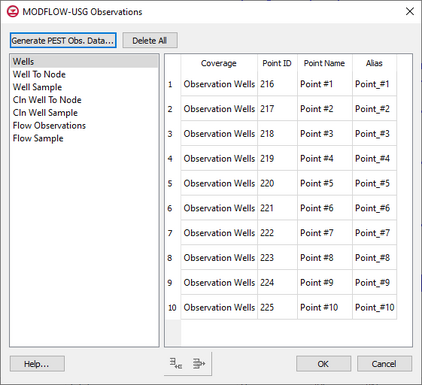
Wells Table
The Wells table provides a list of all of the observation points found in the specified coverages. The table lists the source Coverage Name (CovName), point id (PtId), point name (PtName), and Alias. The Alias field is a string that meets the requirements for "borenames" in the PEST utilities. The alias must be unique (ignoring case), 10 characters or less, and contain no spaces. GMS generates aliases for each of the observation points. If the name of the point satisfies the alias criterion then it is used. None of the data in Wells table can be edited.
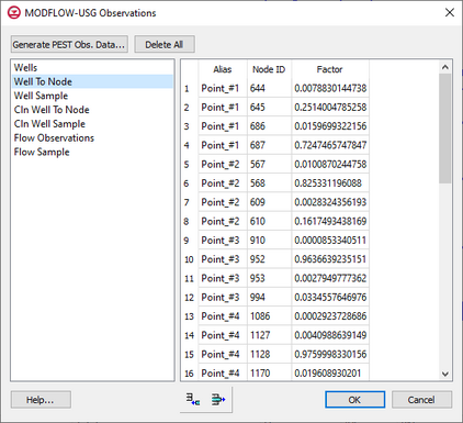
WellToNode Table
The WellToNode table lists the information necessary to interpolate from the UGrid cells to the observation point. The table lists the Alias (same as the Alias listed in the Wells table), id of the UGrid cell (NodeId), and an interpolation factor for the UGrid cell (Factor). The user may edit the values of Alias, NodeId, and Factor as desired. Alias may only be one of the aliases specified in the Wells table. The user may also Add or Delete rows in the table.
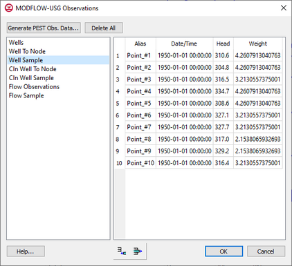
WellSample Table
The WellSample table lists measurements taken at the observation points. The table lists the Alias (same as the Alias listed in the Wells table), the date/time that the measurement was taken (DateTime), and the value of the measurement (Head). When the MODFLOW model is steady state then the DateTime field will contain a value of 1950-01-01 00:00:00. The user may edit the values of Alias, DateTime, and Head as desired. Alias may only be one of the aliases specified in the Wells table. Many different date time formats may be entered into the DataTime field. Regardless of the format enter, the date time will be reformatted into the YYYY-MM-DD HH:MM:SS format.
If the user is not using date time format for the observation data then dates and times will be created using 1950-01-01 00:00:00 as time zero and date times are assigned based on the time units of the MODFLOW-USG simulation.
PEST Utilities for Head Observations
The PEST utility usgmod2obs1.exe is run after a MODFLOW-USG model successfully terminates to calculate the model computed values at the observation points. This utility is run using a batch file called usgmod2obs.bat. This file is written to the same directory as the MODFLOW-USG simulation. The usgmod2obs1.exe utility has several prompts asking the user for input as it runs. The responses to these prompts are written to the file usgmod2obs.in. Three different text files *.obsusg.n2b, *.obsusg.blisting, and *.obsusg.bsamp are written using data from the Wells, WellToNode, and WellSample tables when the MODFLOW-USG simulation is saved. These files are used as part of the input to this utility. The PEST documentation contains the format description for these files. The output from the utility will be a file *.obsusg.bsamp.out that lists the well alias, date time, and head measurement; these are the model computed values at the observation points. The *.obsusg.bsamp.out file is read as part of the MODFLOW-USG solution, used to compute residuals, and used to display calibration targets.
When the MODFLOW-USG model is transient, another batch file: usgmod2obs-mftimes.bat is written. This batch file runs the same usgmod2obs1.exe utility. This batch file will calculate model computed values for the observation points at all of the MODFLOW-USG output time steps. This is done so that when the user views the solution in GMS the model computed value at each observation point at each output time will be available for inspection. An additional file: *.obsusg-mftimes.bsamp is written as input to this batch file. The output of the batch file will be *.obsusg-mftimes.bsamp.out. This file has the same format as *.obsusg.bsamp.out and is also read as part of the MODFLOW-USG solution.
| Name | Description |
|---|---|
| USGMOD2OBS.IN | Input File |
| OBSUSG.N2B | Cell Node Factor File |
| OBSUSG.BLISTING | List of Wells File |
| OBSUSG.BSAMP | Well Sample File |
| OBSUSG.B2B | Bounds File |
| OBSUSG.B2MAP | Well Coordinates File |
| OBSUSG.BWT | Well Weight File |
| OBSUSG | USG Observation Index File |
| Name | Description |
|---|---|
| MFTIMES.BAT | Batch File |
| MFTIMES.BSAMP.OUT | Output File |
| MFTIMES.BSAMP | Sample File |
Flow Observations
The generated flow observation data is stored in 2 tables: FlowObservations and FlowSample. Flow observations may be assigned to points, arcs, arc groups, and polygons that are associated with a MODFLOW boundary condition (drain, general head...).
FlowObs Table
FlowSample Table


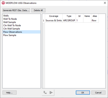
FlowObservations Table
The FlowObservations table provides a list of all of the flow observations found in the specified coverages. The table lists the source Coverage (CovName), the feature object type (Type), the id of the feature object (Id), the name of the feature object (Name), and the Alias. The same rules apply to the Alias in this table as apply to the Alias in the Wells table. None of the data in FlowObservations table can be edited.
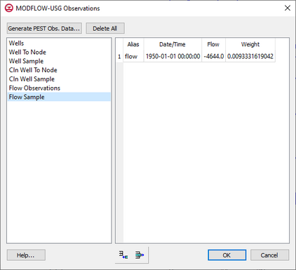
FlowSample Table
The FlowSample table is just like the WellSample table only applied to flow observations.
PEST Utilities for Flow Observations
The PEST utilities usgbud2smp1.exe and smp2smp.exe are run after a MODFLOW-USG model successfully terminates to calculate the model computed flows at the flow observations. This utility is run using batch files called usgbud2smp.bat and usgsmp2smp.bat. These files are written to the same directory as the MODFLOW-USG simulation. The usgbud2smp1.exe utility has several prompts asking the user for input as it runs. The responses to these prompts are written to the file usgbud2smp.in. Two different text files *.obsusgf.b2b and *.obsusgf.fsamp are written using data from the FlowObservations and FlowSample tables when the MODFLOW-USG simulation is saved. These files are used as part of the input to this utility. The PEST documentation contains the format description for these files. The output from the utility will be a file *.obsusgf.samp that lists the flow observation alias, date time, and flow measurement; these are the model computed values at the observations at the model output times. The smp2smp.exe utility does temporal interpolation from the model output times to the observation times and the output from this utility is a file .obsusgf.fsamp.out. The *.obsusgf.fsamp.out file is read as part of the MODFLOW-USG solution, used to compute residuals, and used to display calibration targets.
| Name | Description |
|---|---|
| OBSUSG.FWT | Flow Weight File |
| OBSUSG.FSAMP | Flow Sample File |
| [hide]GMS – Groundwater Modeling System | ||
|---|---|---|
| Modules: | 2D Grid • 2D Mesh • 2D Scatter Point • 3D Grid • 3D Mesh • 3D Scatter Point • Boreholes • GIS • Map • Solid • TINs • UGrids | |
| Models: | FEFLOW • FEMWATER • HydroGeoSphere • MODAEM • MODFLOW • MODPATH • mod-PATH3DU • MT3DMS • MT3D-USGS • PEST • PHT3D • RT3D • SEAM3D • SEAWAT • SEEP2D • T-PROGS • ZONEBUDGET | |
| Aquaveo | ||