GMS:Observations
Observations can be either point observations or flow observations.
Contents
Point Observations
The primary type of field data used in a typical calibration exercise is point observations. Point observations represent values that are measured at some location in the field. Point observations generally correspond to water table elevations measured at observation wells. However, multiple observed values can be defined at each observation point. Observation points are managed in the Map module using the Coverage Setup dialog.
Flow Observations
Flow observations represent gains or losses between aquifers and streams or reservoirs. In addition to point observations, flow observations are an essential part of a calibration exercise for a flow model. If calibration is attempted using point observations only, there may be many combinations of parameters such as hydraulic conductivity and recharge that will result in the same head distribution. Adding one or more flow observations serves to "pin down" the flow quantity resulting in a set of hydraulic conductivities and recharge values that are more likely to be unique.
While the point observation tools are model independent, GMS only supports flow observations for MODFLOW and FEMWATER. With MODFLOW, observed flows are assigned to selected arcs and polygons making up the MODFLOW conceptual model in the Map module. When a MODFLOW solution is imported, the computed flows are read for the arcs and polygons and compared with observed values.
With a FEMWATER simulation, observed values cannot be assigned to objects in the FEMWATER conceptual model. However, when a FEMWATER solution is imported, the computed flows on selected model boundaries can be automatically summed. Comparison of computed vs. observed flows must then be made manually.
Observation Weights
When performing automated parameter estimation, a set of head and flow observations are defined using points, arcs, and polygons in the Map module. When entering the point and flow observations, care should be taken when entering the calibration interval and confidence values. These values are used to determine the weights assigned to each observation in the inverse model. The weight is multiplied by the residual for the observation in the objective function. The weight that is sent to the inverse model input files by GMS is computed as:
Note that GMS will automatically convert from an interval and a confidence to a standard deviation, or directly enter the standard deviation.
Group Weight Multipliers
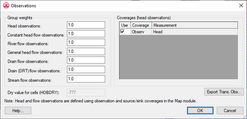
In addition to the individual weight, a group weight can also be assigned. Group weights are assigned using the Group Weight section of the Observations dialog. This dialog is accessed by selecting the Observations command in the MODFLOW menu.
A group weight can be assigned to each of the following observation types:
- Head observations
- Constant head flow observations
- River flow observations
- General head flow observations
- Drain flow observations
- Stream flow observations
Options 2–6 correspond to flow observations that are defined using the Observed flow rate option.
The default value for the group weights is 1.0. The default value can be changed to give a larger influence to a particular observation type. For example, if a particular model had sixteen head observations and one flux observation corresponding to a stream gage, a better solution may be obtained by increasing the flux group weight to give more weight to the stream gage measurement.
Observations Dialog
This dialog (MODFLOW | Observations) is used to manage which coverages that contain MODFLOW observation data will be applied to the current simulation. It is also used to apply group weights. This dialog can only be accessed when observations have been created using the Map Module in a MODFLOW conceptual model.
MODFLOW-USG is different from previous versions of MODFLOW in that it does not support an Observation Process. Computed values at observations for MODFLOW-USG are handled by a series of PEST utilities. The input to these utilities is created in the MODFLOW-USG Observation dialog.
Group Weights
These weights can be used to emphasize (or deemphasize) a type of observation for the simulation.
Coverages
This spreadsheet allows choosing which observation coverages will be used in the current simulation. This can be helpful if there are observations for a site from different times, but only wanting to use one of the times.
Export Trans. Obs.
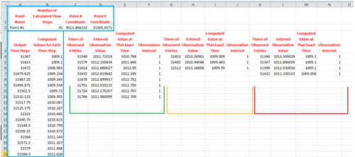
Beginning with version 8.0, this button allows exporting a *.csv (comma separated values) file with transient observation data. This file can be loaded into excel to create plots of the transient observation values vs. the model computed values.
The outputs consist of three main parts:
- The header, which signals the start of a new section. This contains the point name, the point's xy coordinates, and the number of calculated time steps that are printed for it.
- The calculated values, which contains one column with the list of time steps (as determined by the MODFLOW Output Control settings), and one column with the Computed values for each of those times.
- The observed values, which is a section that contains several groupings. Each one has a list of times for which an observation was entered, the entered observation value for that time, and the computed value at that exact time. (This is sometimes different than the output times from the calculated list, so it provides an exact value to compare, instead of requiring an estimation based on the output list.)
Confidence Interval and Standard Deviation
The interval and standard deviation are related by the following equation:
where sd is the standard deviation, CI is the confidence interval, and z is the the "z statistic" based on the specified confidence and the normal distribution. Enter an interval and confidence, and the standard deviation will be computed; or enter a standard deviation and confidence, and the interval will be computed.
In practical terms entering an interval (or standard deviation) and confidence is an indication of how much error is believed to be associated with the observed value.
The standard deviation becomes important when using an inverse model. The weight assigned to each of the observations points is a function of the standard deviation. This weight is used in the objective function that the inverse model tries to minimize. An observation point with a small standard deviation will have a greater influence on the objective function than a point with a large standard deviation.
Enter an interval (or standard deviation) and confidence in the Properties dialog. Although these values are rarely quantified the following examples may prove helpful.
For example, if having the following set of head measurements for one observation well:
Date Head May 10, 1998 55.0 July 10, 1998 50.5 September 5, 1998 48.6 November 15, 1998 49.1 February 2, 1999 50.8 March 12, 1999 54.0 April 1, 1999 57.2
The mean of the data is 52.17 and the standard deviation is 3.25. Enter this standard deviation and a confidence of 95%.
Many times there is not this much data available. Usually there will only be one measured value. In this case use engineering judgement to estimate an interval or standard deviation. For example, if there is a single head measurement of 45.7 ft and it is believed that observation is accurate to within 1 foot, then enter 1 foot as the interval.
See also
| [hide]GMS – Groundwater Modeling System | ||
|---|---|---|
| Modules: | 2D Grid • 2D Mesh • 2D Scatter Point • 3D Grid • 3D Mesh • 3D Scatter Point • Boreholes • GIS • Map • Solid • TINs • UGrids | |
| Models: | FEFLOW • FEMWATER • HydroGeoSphere • MODAEM • MODFLOW • MODPATH • mod-PATH3DU • MT3DMS • MT3D-USGS • PEST • PHT3D • RT3D • SEAM3D • SEAWAT • SEEP2D • T-PROGS • ZONEBUDGET | |
| Aquaveo | ||


