|
|
| (31 intermediate revisions by the same user not shown) |
| Line 1: |
Line 1: |
| | __NOINDEX__ |
| | {{Version GMS 10.4}} |
| {{UGrid links}} | | {{UGrid links}} |
| | __TOC__ |
| UGrid [[GMS:Datasets|datasets]] can be interpolated to other UGrids similar to how scatter point datasets can be interpolated to other objects. The '''Interpolate To''' command is found in the right-click menu of the UGrid dataset to be interpolated to another UGrid. This command opens the ''Interpolate UGrid to UGrid'' dialog: | | UGrid [[GMS:Datasets|datasets]] can be interpolated to other UGrids similar to how scatter point datasets can be interpolated to other objects. The '''Interpolate To''' command is found in the right-click menu of the UGrid dataset to be interpolated to another UGrid. This command opens the ''Interpolate UGrid to UGrid'' dialog: |
|
| |
|
| Line 23: |
Line 26: |
| **''Points'' – Specifies the new dataset will be located at the points. | | **''Points'' – Specifies the new dataset will be located at the points. |
| **''Cells'' – Specifies the new dataset will be located at the cells. | | **''Cells'' – Specifies the new dataset will be located at the cells. |
| | |
| | ==UGrid Interpolation Options== |
| | Clicking the '''Options''' button will open a dialog specific to the interpolation method being used. |
| | ===Linear=== |
| | The Linear interpolation scheme uses data points that are first triangulated to form a network of triangles. See [[GMS:UGrid Linear Interpolation|UGrid Linear Interpolation]] for more details. |
| | |
| | ===Inverse Distance Weighted=== |
| | Inverse Distance Weighted (IDW) is one of the most commonly used techniques for interpolation of point data. Its methods are based on the assumption that the interpolating surface should be influenced most by the nearby points and less by the more distant points. See [[GMS:UGrid Inverse Distance Weighted Interpolation|UGrid Inverse Distance Weighted Interpolation]] for more details. |
| | |
| | ===Natural Neighbor=== |
| | Natural neighbor interpolation is based on the Thiessen polygon network of the point data. The Thiessen polygon network can be constructed from the Delaunay triangulation of a set of points. A Delaunay triangulation is a network of triangles that has been constructed so that the Delaunay criterion has been satisfied. As with IDW interpolation, the nodal functions can be either constants, gradient planes, or quadratics. See [[GMS:UGrid Natural Neighbor Interpolation|UGrid Natural Neighbor Interpolation]] for more details. |
| | |
| | ===Kriging=== |
| | Kriging is based on the assumption that the parameter being interpolated can be treated as a regionalized variable. A regionalized variable is intermediate between a truly random variable and a completely deterministic variable because it varies in a continuous manner from one location to the next. Therefore points that are near each other have a certain degree of spatial correlation, but points that are widely separated are statistically independent. Kriging is a set of linear regression routines which minimize estimation variance from a predefined covariance model. |
| | |
| | See [[GMS:UGrid Kriging Interpolation|UGrid Kriging Interpolation]] for more details. |
| | |
| | ===Advanced=== |
| | [[File:Interplate-Advanced.png|thumb|350 px|The ''Interpolate – Advanced'' dialog]] |
| | The ''Interpolate – Advanced'' dialog is accessed through the '''Advanced''' on the interpolation method dialogs. Options in this dialog include: |
| | *''Anisotropy'' – Options in this section allow taking into account for directional tendencies in the original dataset. |
| | **''Horizontal anisotropy'' |
| | **''Azimuth'' – Sets angle of degrees between the projected vector and a reference vector on the reference plane. |
| | **''Vertical Anisotropy (1/z mag)'' – Available with the 3D option. Vertical anisotropy is 1 over the Z scale. |
| | *''Extrapolation'' |
| | **''Value'' |
| | **''Assign extrapolation value to hidden objects'' — Assigns the default extrapolation value to all cells that are hidden using the '''Hide''' command in the ''Display | Visibility'' menu. |
|
| |
|
| ==Points vs. Cells== | | ==Points vs. Cells== |
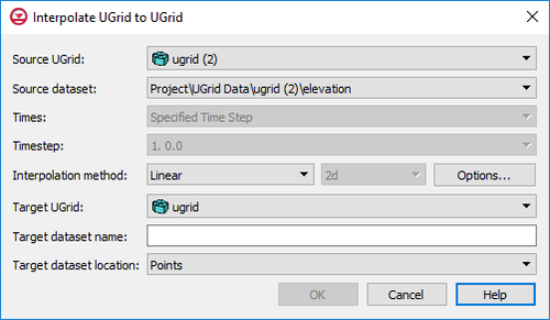
UGrid datasets can be interpolated to other UGrids similar to how scatter point datasets can be interpolated to other objects. The Interpolate To command is found in the right-click menu of the UGrid dataset to be interpolated to another UGrid. This command opens the Interpolate UGrid to UGrid dialog:

Interpolate UGrid to UGrid dialog
This dialog allows selecting the interpolation options to use, and the UGrid to interpolate to. See Interpolation for more information on interpolation. Options include:
- Source UGrid – The drop-down menu here will display a list of all available UGrids. Select the UGrid containing the source dataset.
- Source dataset – The drop-down menu will display a list of all available datasets under the source UGrid. Select the dataset to use for interpolation.
- Times – If the source dataset is transient, time steps should be specified. Options include:
- "Specified Time Step" – This option will use the select time step in the next field.
- "All Times" – This option will use all time steps available in the source dataset.
- Interpolation method – This section specifies which interpolation process will be used.
- Linear – Uses data points that are first triangulated to form a network of triangles. The Options button for this method will bring up the Interpolate – Linear dialog where the interpolation values can be truncated or the Clough-Tocher method can be applied.
- Inverse distance weighted – Creates an interpolated surface that is a weighted average of the point data; the weight assigned to each point diminishes as the distance to the interpolation location increases. The Options button next to this option will bring up either the 2D IDW Interpolation Options dialog or the 3D IDW Interpolation Options dialog.
- Natural neighbor – Based on the Thiessen polygon network of the point data. The Options button next to this option will bring up the Natural Neighbor Options dialog.
- Kriging – Based on the assumption that the parameter being interpolated can be treated as a regionalized variable. The Options button next to this option will bring up the Kriging Options dialog.
- Dimension – Options in this drop-down determine whether the interpolation will be two-dimensional or three dimensional.
- 2D – Designates the interpolation as two-dimensional data. This is the default interpolation method.
- 3D – Specified the interpolation as three-dimensional data. Only the inverse distance weighted and Kriging options are available with this method.
- Target UGrid – The drop-down menu will contain a list of available UGrids where the source dataset can be interpolated.
- Target dataset name – Enter a name for the new dataset that will appear under the target UGrid.
- Target dataset location – Specifies where the new dataset will be located: at the points or at the cells.
- Points – Specifies the new dataset will be located at the points.
- Cells – Specifies the new dataset will be located at the cells.
UGrid Interpolation Options
Clicking the Options button will open a dialog specific to the interpolation method being used.
Linear
The Linear interpolation scheme uses data points that are first triangulated to form a network of triangles. See UGrid Linear Interpolation for more details.
Inverse Distance Weighted
Inverse Distance Weighted (IDW) is one of the most commonly used techniques for interpolation of point data. Its methods are based on the assumption that the interpolating surface should be influenced most by the nearby points and less by the more distant points. See UGrid Inverse Distance Weighted Interpolation for more details.
Natural Neighbor
Natural neighbor interpolation is based on the Thiessen polygon network of the point data. The Thiessen polygon network can be constructed from the Delaunay triangulation of a set of points. A Delaunay triangulation is a network of triangles that has been constructed so that the Delaunay criterion has been satisfied. As with IDW interpolation, the nodal functions can be either constants, gradient planes, or quadratics. See UGrid Natural Neighbor Interpolation for more details.
Kriging
Kriging is based on the assumption that the parameter being interpolated can be treated as a regionalized variable. A regionalized variable is intermediate between a truly random variable and a completely deterministic variable because it varies in a continuous manner from one location to the next. Therefore points that are near each other have a certain degree of spatial correlation, but points that are widely separated are statistically independent. Kriging is a set of linear regression routines which minimize estimation variance from a predefined covariance model.
See UGrid Kriging Interpolation for more details.
Advanced

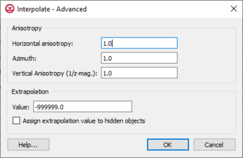
The
Interpolate – Advanced dialog
The Interpolate – Advanced dialog is accessed through the Advanced on the interpolation method dialogs. Options in this dialog include:
- Anisotropy – Options in this section allow taking into account for directional tendencies in the original dataset.
- Horizontal anisotropy
- Azimuth – Sets angle of degrees between the projected vector and a reference vector on the reference plane.
- Vertical Anisotropy (1/z mag) – Available with the 3D option. Vertical anisotropy is 1 over the Z scale.
- Extrapolation
- Value
- Assign extrapolation value to hidden objects — Assigns the default extrapolation value to all cells that are hidden using the Hide command in the Display | Visibility menu.
Points vs. Cells
UGrids can have datasets associated with both cells and points. Thus there is an option to specify where the new dataset will be located: at the points or at the cells.
