GMS includes an interpolation option associated with the 2D scatter point module called Gaussian Sequential Simulation (GSS). This option is used to generate a set of scalar datasets (Gaussian fields) using a Gaussian sequential simulation. This is somewhat similar to indicator kriging or T-PROGS in that it generates a set of equally probable results which exhibit heterogeneity and are conditioned to values at scatter points. However, the resulting arrays are floating point scalar datasets, rather than the integer arrays produced by T-PROGS and indicator kriging.
The results of a GSS can be used in combination with the new Multiplier Array option for parameters. It is now possible to associate one or more scalar datasets with an array-based parameter. When MODFLOW is executed, the parameter starting value is multiplied by the dataset to produce the input array. This makes it possible to use the results of the Gaussian sequential simulation as input for parameter fields for a stochastic (Monte Carlo) simulation.
Gaussian Simulations
The new GSS tool is based on the FIELDGEN code developed by John Doherty. John Doherty describes GSS as follows:
The process of stochastic field generation by sequential simulation is very easy to understand. At each field point an expected field value and a field standard deviation pertaining to that point are first determined. These are calculated through kriging from points to which field values have already been assigned, as well as from points at which conditioning data exists (if available). Using the expected value and standard deviation calculated in this way, a random field value is generated based on the assumption of a Gaussian probability distribution. The field value thus obtained can then be used in generating expected values and standard deviations at other field points at which field generation then takes place in the same way.
GSS is a form of Kriging but it is listed in the GMS interface as a new interpolation scheme. This new option will differ from Kriging in the following ways:
- GSS uses the FIELDGEN utility developed by John Doherty to perform the interpolation rather than the GSLIB code used by kriging. FIELDGEN is a modified version of the sgsim utility in GSLIB so many of the options are quite similar to those used for normal kriging.
- As is the case with T-PROGS, enter the number of desired simulations and FIELDGEN produces N arrays, rather than one array.
- It can only be used for 2D interpolation and it will only work when interpolating to 3D cell-centered grids.
- It can work with or without a scatter point set. If a scatter point set is provided, the resulting fields are conditioned to the values at the scatter points. Otherwise define a mean and a variogram and the values are randomly generated.
Gaussian Simulation Options
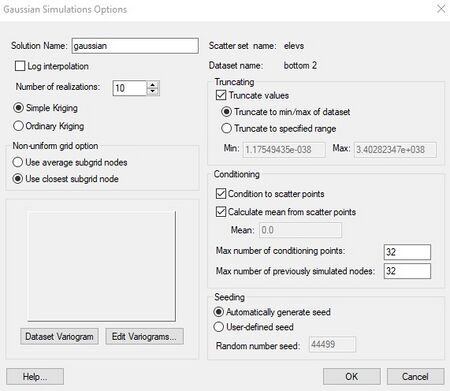
The first step in setting up a GSS is to import a set of scatter points with the values to which to condition the simulation. This step can be skipped if there is no conditioning data. The next step is to select the Gaussian Simulation Options command in the Interpolation menu in the 2D Scatter Point module. This brings up the following dialog:

Example of the
Gaussian Simulations Options dialog.
The Solution name at the top is the name that will be applied to the set of Gaussian fields. The Number of realizations item is the desired number of Gaussian fields. The original GSLIB code was designed to work with uniform grids (constant cell sizes). The Non-uniform grid option controls how the data are converted to a non-uniform grid (if necessary). The Edit Variogram button should be selected to set up a model variogram using the GMS Variogram Editor. A model variogram must be defined whether or not there are scatter points for conditioning.
Running the Simulation
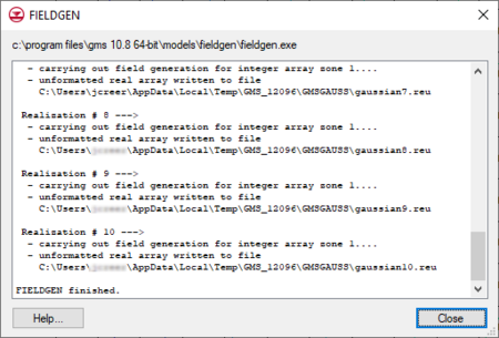
Once the GSS options are selected, the next step is to run the simulation. This is accomplished by selecting the Run Gaussian Simulation command in the Interpolation menu. During the simulation, a window displays the progress of the simulation:

Example of the Gaussian
FIELDGEN wrapper dialog.
Viewing the Results
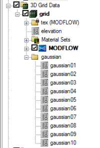
Once the simulation is finished, a new folder appears in the Project Explorer window which has the name of the simulation and contains a set of dataset arrays:
Clicking on each dataset icon  makes it the active dataset for contouring. The dataset properties can be viewed by double-clicking on the icon
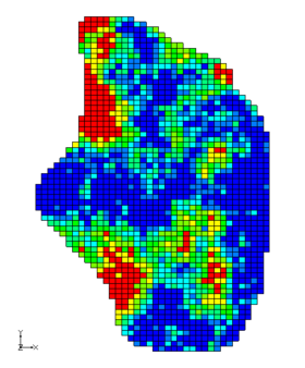
  . The following image represents a sample Gaussian realization:
