GMS:Interpolation Commands
Once a 3D interpolation scheme has been selected and the appropriate parameters for the selected scheme have been input, the dataset of the active scatter point set can be interpolated to another object. During the interpolation process, a new dataset is constructed for the target object containing the interpolated values. A separate interpolation command is provided for interpolating to each of the target objects. The interpolation commands are found in the Interpolation menu. The commands in this menu are as follows:
- Interpolation Options
- Opens the Interpolation Options dialog to change the interpolation method.
- Interpolate → Active TIN
- Interpolates to the vertices of the active TIN.
- Interpolate → 2D Mesh
- Interpolates to the nodes of the 2D finite element mesh.
- Interpolate → 2D Grid
- Interpolates to the 2D finite difference grid. The interpolation is done either to the grid nodes or to the grid cell centers depending on whether the grid is a mesh-centered or cell-centered grid. (See 2D Grid Types.)
- Interpolate → 3D Mesh
- Interpolates to the nodes of the 3D finite element mesh.
- Interpolate → 3D Grid
- Interpolates to the 3D finite difference grid. The interpolation is done either to the grid nodes or to the grid cell centers depending on whether the grid is a mesh-centered or cell-centered grid. (See 2D Grid Types.)
- Interpolate → MODFLOW Layers
- The Interpolate to MODFLOW Layers command allows interpolating from 2D scatter data to MODFLOW data: top and bottom layer elevations, LPF array data (HK, VK, etc.), recharge.
- Interpolate → UGrid
- Interpolates to the cells of the active UGrid.
- Gaussian Simulation Options
- Gaussian Sequential Simulation (GSS) is a form of Kriging that can only be used for 2D interpolation and only works when interpolating to 3D cell-centered grids.
- Jackknifing
- Interpolates the active scatter point set to itself using the currently selected interpolation scheme. 3D jackknifing is identical to 2D jackknifing.
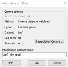
When one of the interpolation commands is selected, the Interpolate→Object dialog appears. This dialog shows the interpolation being used and has an option to bring up the Interpolation Options dialog to change the interpolation method. The Interpolated dataset name can also be specified for the new dataset being generated.
See also
GMS – Groundwater Modeling System | ||
|---|---|---|
| Modules: | 2D Grid • 2D Mesh • 2D Scatter Point • 3D Grid • 3D Mesh • 3D Scatter Point • Boreholes • GIS • Map • Solid • TINs • UGrids | |
| Models: | FEFLOW • FEMWATER • HydroGeoSphere • MODAEM • MODFLOW • MODPATH • mod-PATH3DU • MT3DMS • MT3D-USGS • PEST • PHT3D • RT3D • SEAM3D • SEAWAT • SEEP2D • T-PROGS • ZONEBUDGET | |
| Aquaveo | ||
