WMS:Computation of Interpolation Weights

When computing the interpolation weights, three options are available for determining which points are included in the subset of points used to compute the weights and perform the interpolation: subset, all points, and enclosing triangle.

Subset of Points

If the Use subset of points option is chosen, the Subset Definition dialog can be used to define a local subset of points.

All Points

If the Use all points option is chosen, a weight is computed for each point and all points are used in the interpolation.

Enclosing Triangle

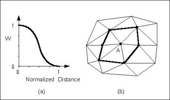
The Use vertices of enclosing triangle method makes the interpolation process a local scheme by taking advantage of TIN topology (Franke & Nielson, 1980). With this technique, the subset of points used for interpolation consists of the three vertices of the triangle containing the interpolation point. The weight function or blending function assigned to each scatter point is a cubic S-shaped function as shown in part a of the figure below. The fact that the slope of the weight function tends to unity at its limits ensures that the slope of the interpolating surface is continuous across triangle boundaries.

(a) S-Shaped Weight Function and (b) Delauney Point Group for Point A.

The influence of the weight function extends over the limits of the Delauney point group of the scatter point. The Delauney point group is the "natural neighbors" of the scatter point, and the perimeter of the group is made up of the outer edges of the triangles that are connected to the scatter point as shown in part b. The weight function varies from a weight of unity at the scatter point to zero at the perimeter of the group. For every interpolation point in the interior of a triangle there are three nonzero weight functions (the weight functions of the three vertices of the triangle). For a triangle T with vertices i, j, and k, the weights for each vertex are determined as follows:

$w_{i}(x,y)=b_{i}^{2}(3-2b_{i})+3{\frac {b_{i}^{2}b_{j}b_{k}}{b_{i}b_{j}+b_{i}b_{k}+b_{j}b_{k}}}$

$\left\{b_{j}\left[{\frac {\|e_{i}\|^{2}+\|e_{k}\|^{2}-\|e_{j}\|^{2}}{\|e_{k}\|^{2}}}\right]+b_{k}\left[{\frac {\|e_{i}\|^{2}+\|e_{j}\|^{2}-\|e_{k}\|^{2}}{\|e_{j}\|^{2}}}\right]\right\}$

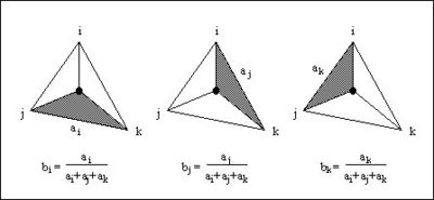
where ||ei|| is the length of the edge opposite vertex i, and b_i, b_j, b_k are the area coordinates of the point (x,y) with respect to triangle T. Area coordinates are coordinates that describe the position of a point within the interior of a triangle relative to the vertices of the triangle. The coordinates are based solely on the geometry of the triangle. Area coordinates are sometimes called "barycentric coordinates." The relative magnitude of the coordinates corresponds to area ratios as shown below:

Barycentric coordinates for a point in a triangle.

The xy coordinates of the interior point can be written in terms of the xy coordinates of the vertices using the area coordinates as follows:

$x=b_{i}x_{i}+b_{j}x_{j}+b_{k}x_{k}^{}$

$y=b_{i}y_{i}+b_{j}y_{j}+b_{k}y_{k}^{}$

$1.0=b_{i}+b_{j}+b_{k}^{}$

Solving the above equations for $b_{i}$, $b_{j}$, and $b_{k}$ yields:

$b_{i}{\frac {1}{2A}}[(x_{j}y_{k}-x_{k}y_{j})+(y_{j}-y_{k})x+(x_{k}-x_{j})y]$

$b_{j}{\frac {1}{2A}}[(x_{k}y_{i}-x_{i}y_{k})+(y_{k}-y_{i})x+(x_{i}-x_{k})y]$

$b_{k}{\frac {1}{2A}}[(x_{i}y_{j}-x_{j}y_{i})+(y_{i}-y_{j})x+(x_{j}-x_{i})y]$

$A={\frac {1}{2}}(x_{i}y_{j}+x_{j}y_{k}+x_{k}y_{i}-y_{i}x_{j}-y_{j}x_{k}-y_{k}x_{i})$

Using the weight functions defined above, the interpolating surface at points inside a triangle is computed as:

$F(x,y)=w_{i}(x,y)Q_{i}(x,y)+w_{j}(x,y)Q_{j}(x,y)+w_{k}(x,y)Q_{k}^{}(x,y)$

where w_i, w_j, and w_k are the weight functions and Q_i, Q_j, and Q_k are the nodal functions for the three vertices of the triangle.

Related Topics

• Inverse Distance Weighted Interpolation
• Subset Definition
• Shepard's Method
• Gradient Plane Nodal Functions
• Quadratic Nodal Functions