WMS:OC Rational Job Control: Difference between revisions
From XMS Wiki
Jump to navigationJump to search
No edit summary |
No edit summary |
||
| Line 1: | Line 1: | ||
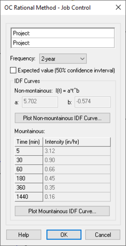
[[Image:OC_Reational_Job_control.JPG|thumb|250 px|''OC Rational Method – Job Control'' dialog]] | [[Image:OC_Reational_Job_control.JPG|thumb|250 px|''OC Rational Method – Job Control'' dialog]] | ||
The ''Job Control'' parameters include all of the universal data necessary to run an Orange County analysis that are not a part of a basin, reach, or reservoir. The following are the specific parameters defined as part of job control: | The ''OC Rational Method – Job Control'' parameters include all of the universal data necessary to run an Orange County analysis that are not a part of a basin, reach, or reservoir. The following are the specific parameters defined as part of job control: | ||
*'''Units''' – By default Orange County performs computations in English units, however metric unit calculations can be specified. | *'''Units''' – By default Orange County performs computations in English units, however metric unit calculations can be specified. | ||
Revision as of 15:24, 16 October 2017
The OC Rational Method – Job Control parameters include all of the universal data necessary to run an Orange County analysis that are not a part of a basin, reach, or reservoir. The following are the specific parameters defined as part of job control:
- Units – By default Orange County performs computations in English units, however metric unit calculations can be specified.
- Frequency – Select the return period of the design storm. Non-mountainous and mountainous IDF curve values are updated based on this selection. Enter IDF curve values for the 500-yr storm.
- Expected Value – Toggle this check box on to do an expected value analysis. IDF curves and losses will be automatically updated for each sub-area if they have already been computed.
IDF Curves
IDF (intensity-duration-frquency) curves in Orange County are calculated differently depending on the location of the analysis. This section is subdivided into non-mountainous (areas below 2000 feet) and mountainous (areas above 2000 feet) regions.
- Non-mountainous – The IDF curves are generated using a regression equation I = atb where:
- I – Rainfall intensity (in/hr, mm/hr)
- t – Duration (min)
- a, b – Regression equation coefficients
- Mountainous – The IDF curves are generated by interpolating between known intensities at specified time values.
Related Topics
WMS – Watershed Modeling System | ||
|---|---|---|
| Modules: | Terrain Data • Drainage • Map • Hydrologic Modeling • River • GIS • 2D Grid • 2D Scatter |  |
| Models: | CE-QUAL-W2 • GSSHA • HEC-1 • HEC-HMS • HEC-RAS • HSPF • MODRAT • NSS • OC Hydrograph • OC Rational • Rational • River Tools • Storm Drain • SMPDBK • SWMM • TR-20 • TR-55 | |
| Toolbars: | Modules • Macros • Units • Digitize • Static Tools • Dynamic Tools • Drawing • Get Data Tools | |
| Aquaveo | ||
