GMS:T-PROGS: Difference between revisions
From XMS Wiki
Jump to navigationJump to search
| (10 intermediate revisions by 3 users not shown) | |||
| Line 1: | Line 1: | ||
{{Infobox Model | | {{Infobox Model | | ||
|name= T-PROGS | |name= T-PROGS | ||
|screenshot= Image:Matset. | |screenshot= Image:Matset.png | ||
|model_type= transition probability geostatistics on borehole data | |model_type= transition probability geostatistics on borehole data | ||
|developer= Steven Carle | |developer= Steven Carle | ||
| Line 9: | Line 9: | ||
{{T-PROGS Links}} | {{T-PROGS Links}} | ||
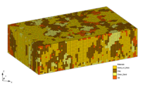
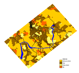
GMS includes an interface to the T-PROGS software developed by Steven Carle. The T-PROGS software is used to perform transition probability geostatistics on borehole data. The output of the T-PROGS software is a set of N [[GMS:Material Set|material sets]] on a 3D grid. Each of the material sets is conditioned to the borehole data and the materials proportions and transitions between the boreholes | GMS includes an interface to the T-PROGS (Transition PRObability GeoStatistical) software developed by Steven Carle. The T-PROGS software is used to perform transition probability geostatistics on borehole data. The output of the T-PROGS software is a set of N [[GMS:Material Set|material sets]] on a 3D grid. Each of the material sets is conditioned to the borehole data and the materials proportions and transitions between the boreholes following the trends observed in the borehole data. These material sets can be used for [[GMS:Stochastic Modeling#Stochastic Applications|stochastic simulations]] with MODFLOW. A sample material set generated by the T-PROGS software is shown below. This software can also be used to generate multiple input datasets for the [[GMS:HUF Package|HUF package]]. | ||
The T-PROGS model can be added to a [http://www.aquaveo.com/software/gms-pricing paid edition] of GMS. | The T-PROGS model can be added to a [http://www.aquaveo.com/software/gms-pricing paid edition] of GMS. | ||
| Line 30: | Line 30: | ||
<!--[[Image:t-progs_eq1.png]] | <!--[[Image:t-progs_eq1.png]] | ||
<math>t_{jk}(\mathbf{h})= \text{Pr}\{k \text{ occurs at } \mathbf{x} + \mathbf{h}\ |\ j \text{ occurs at } \mathbf{x}\}</math>--> | <math>t_{jk}(\mathbf{h})= \text{Pr}\{k \text{ occurs at } \mathbf{x} + \mathbf{h}\ |\ j \text{ occurs at } \mathbf{x}\}</math>--> | ||
[[image:tprogseq1.jpg]]<div style="float: right;"><ref> | :[[image:tprogseq1.jpg]]<div style="float: right;"><ref> | ||
{{citation | {{citation | ||
|last=Carle | |last=Carle | ||
| Line 47: | Line 47: | ||
<!-- [[Image:t-progs_eq2.png]] | <!-- [[Image:t-progs_eq2.png]] | ||
<math>\mathbf{T}(h_\phi)=\text{exp}(\mathbf{R}_{\phi}h_\phi)</math>--> | <math>\mathbf{T}(h_\phi)=\text{exp}(\mathbf{R}_{\phi}h_\phi)</math>--> | ||
[[image:tprogseq2.jpg]]<div style="float: right;"><ref> | :[[image:tprogseq2.jpg]]<div style="float: right;"><ref> | ||
{{citation | {{citation | ||
|last=Carle | |last=Carle | ||
| Line 60: | Line 60: | ||
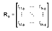
where ''h'' denotes a lag in the direction ''Φ'', and ''RΦ'' denotes a transition rate matrix | where ''h'' denotes a lag in the direction ''Φ'', and ''RΦ'' denotes a transition rate matrix | ||
[[Image:rate_matrix. | :[[Image:rate_matrix.png]] | ||
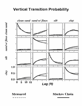
with entries ''r<sub>jk</sub>,f'' representing the rate of change from category ''j'' to category ''k'' (conditional to the presence of ''j'') per unit length in the direction ''Φ''. The transition rates are adjusted to ensure a good fit between the Markov Chain model and the observed transition probability data. | with entries ''r<sub>jk</sub>,f'' representing the rate of change from category ''j'' to category ''k'' (conditional to the presence of ''j'') per unit length in the direction ''Φ''. The transition rates are adjusted to ensure a good fit between the Markov Chain model and the observed transition probability data. | ||
| Line 67: | Line 67: | ||
In the final phase of setting up a transition probability analysis using T-PROGS, the modeler creates a grid, specifies the number of model instances (N), and launches the TSIM utility. The TSIM code uses the 3D Markov chain to formulate both indicator cokriging equations and an objective function for simulated annealing. It generates [[GMS:Stochastic Modeling#Stochastic Applications|stochastic simulations]] using a combination of modified versions of the GSLIB codes SISIM and ANNEAL. | In the final phase of setting up a transition probability analysis using T-PROGS, the modeler creates a grid, specifies the number of model instances (N), and launches the TSIM utility. The TSIM code uses the 3D Markov chain to formulate both indicator cokriging equations and an objective function for simulated annealing. It generates [[GMS:Stochastic Modeling#Stochastic Applications|stochastic simulations]] using a combination of modified versions of the GSLIB codes SISIM and ANNEAL. | ||
TPROGS allows roughly up to 3.5 million cells to be included in a simulation. Model instabilities may appear if more that 3.5 million cells are used. | |||
==T-PROGS Materials== | ==T-PROGS Materials== | ||
| Line 74: | Line 76: | ||
|} | |} | ||
When having selected the '''New Simulation''' command to initialize a T-PROGS simulation, the ''T-PROGS Boreholes'' dialog appears. Here | When having selected the '''New Simulation''' command to initialize a T-PROGS simulation, the ''T-PROGS Boreholes'' dialog appears. Here select to use all boreholes or only the boreholes in a particular folder. | ||
===HGUs=== | ===HGUs=== | ||
| Line 80: | Line 82: | ||
===Material List=== | ===Material List=== | ||
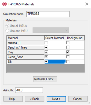
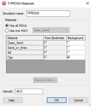
If boreholes do not exist in the model, an unconditioned simulation will be generated. In this case, in the ''T-PROGS Materials'' dialog | If boreholes do not exist in the model, an unconditioned simulation will be generated. In this case, in the ''T-PROGS Materials'' dialog select the materials to be used and a corresponding background material. The upper part of the dialog lists the materials in the boreholes. The first column of toggles indicates which materials are to be used in the analysis. By default, all materials associated with the boreholes are selected. These toggles are necessary since it is possible that there may be materials defined in the materials list that are not associated with boreholes. The second column in the top section of the dialog lists the background material. By default, the material type that had the predominant occurrence in the boreholes (greatest proportion) is marked as the background material. When defining the transition probability data in the next section, the input parameters do not need to be edited for the background material. The parameters for this material are automatically adjusted to balance the equations. | ||
===Background Material=== | ===Background Material=== | ||
| Line 99: | Line 101: | ||
==Generating Material Sets with T-PROGS== | ==Generating Material Sets with T-PROGS== | ||
The underlying equations solved by the T-PROGS software require an orthogonal grid with constant cell dimensions (X, Y, and Z). The delta X values can be different from the delta Y and delta Z values, and the delta Y values can be different from the delta Z values, but all cells must have the same change in X, Y, and Z dimensions. The MODFLOW model is capable of using the [[GMS:LPF Package|Layer Property Flow (LPF) | The underlying equations solved by the T-PROGS software require an orthogonal grid with constant cell dimensions (X, Y, and Z). The delta X values can be different from the delta Y and delta Z values, and the delta Y values can be different from the delta Z values, but all cells must have the same change in X, Y, and Z dimensions. The MODFLOW model is capable of using the [[GMS:LPF Package|Layer Property Flow (LPF) package]] with the ''Material ID'' option for assigning aquifer properties. With this option, each cell in the grid is assigned a material ID and the aquifer properties (Kh, Kv, etc.) associated with each material are automatically assigned to the layer data arrays for the LPF package when the MODFLOW files are saved. The T-PROGS software generates multiple material sets (arrays of material IDs), each of which represents a different realization of the aquifer heterogeneity. When running a MODFLOW simulation in [[GMS:Stochastic Modeling#Stochastic Applications|stochastic mode]], GMS automatically loads each of the N material sets generated by the T-PROGS software and saves N different sets of MODFLOW input files. The N solutions resulting from these simulations can be read into GMS and used to perform [[GMS:Risk_Analysis_Wizard|risk analyses]] such as probabilistic capture zone delineation. | ||
=== One-Layer MODFLOW Grids === | === One-Layer MODFLOW Grids === | ||
| Line 114: | Line 116: | ||
Using transition probability geostatistics with MODFLOW models results in two basic limitations. First, the underlying stochastic algorithms used by the T-PROGS software are formulated such that the MODFLOW grid must have uniform row, column, and layer widths. The row width can be different from the column width, but each row must have the same width. This results in a uniform orthogonal grid. While MODFLOW grids are orthogonal in x and y, the layer thickness is allowed to vary on a cell-by-cell basis. This makes it possible for the layer boundaries to accurately model the ground surface and the tops and bottoms of aquifer units. If a purely orthogonal grid is used, irregular internal and external layer boundaries must be simulated in a stair-step fashion either by varying material properties or by activating/inactivating cells via the IBOUND array. A second limitation is that in order to get a high level of detail in the simulated heterogeneity, the grid cell dimensions are generally kept quite small. This can result in difficulties in the vertical dimension. The large number of layers with small layer thicknesses near the top of the model generally ensures that many of the cells in this region will be at or above the computed water table elevation (for simulations involving unconfined aquifers). As a result, these cells will undergo many of the numerical instabilities and increased computational effort issues associated with cell wetting and drying. | Using transition probability geostatistics with MODFLOW models results in two basic limitations. First, the underlying stochastic algorithms used by the T-PROGS software are formulated such that the MODFLOW grid must have uniform row, column, and layer widths. The row width can be different from the column width, but each row must have the same width. This results in a uniform orthogonal grid. While MODFLOW grids are orthogonal in x and y, the layer thickness is allowed to vary on a cell-by-cell basis. This makes it possible for the layer boundaries to accurately model the ground surface and the tops and bottoms of aquifer units. If a purely orthogonal grid is used, irregular internal and external layer boundaries must be simulated in a stair-step fashion either by varying material properties or by activating/inactivating cells via the IBOUND array. A second limitation is that in order to get a high level of detail in the simulated heterogeneity, the grid cell dimensions are generally kept quite small. This can result in difficulties in the vertical dimension. The large number of layers with small layer thicknesses near the top of the model generally ensures that many of the cells in this region will be at or above the computed water table elevation (for simulations involving unconfined aquifers). As a result, these cells will undergo many of the numerical instabilities and increased computational effort issues associated with cell wetting and drying. | ||
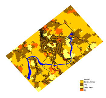
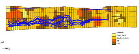
[[Image:huf_sample. | [[Image:huf_sample.png|thumb|right|475 px|Sample HUF stratigraphy data generated by the T-PROGS software. Blue lines represent particle path lines and water table.]] | ||
The Hydrogeologic Unit Flow (HUF) package released with MODFLOW 2000 makes it possible to overcome both of these limitations resulting in a powerful mechanism for incorporating transition probability geostatistics in MODFLOW simulations. With the HUF package, the modeler is allowed to input the vertical component of the stratigraphy in a grid-independent fashion. The stratigraphy data are defined using a set of elevation and thickness arrays. The first array defines the top elevation of the model. The remaining arrays define the thicknesses of a series of hydrogeologic units, starting at the top and progressing to the bottom of the model. For each array of thicknesses, many of the entries in the array may be zero. This makes it possible to simulate complex heterogeneity, including pinchouts and embedded lenses that would be difficult to simulate with the LPF and BCF packages. | The Hydrogeologic Unit Flow (HUF) package released with MODFLOW 2000 makes it possible to overcome both of these limitations resulting in a powerful mechanism for incorporating transition probability geostatistics in MODFLOW simulations. With the HUF package, the modeler is allowed to input the vertical component of the stratigraphy in a grid-independent fashion. The stratigraphy data are defined using a set of elevation and thickness arrays. The first array defines the top elevation of the model. The remaining arrays define the thicknesses of a series of hydrogeologic units, starting at the top and progressing to the bottom of the model. For each array of thicknesses, many of the entries in the array may be zero. This makes it possible to simulate complex heterogeneity, including pinchouts and embedded lenses that would be difficult to simulate with the LPF and BCF packages. | ||
| Line 129: | Line 131: | ||
[[Category:T-PROGS Dialogs]] | [[Category:T-PROGS Dialogs]] | ||
[[Category:GMS Stochastic Modeling Dialogs]] | [[Category:GMS Stochastic Modeling Dialogs]] | ||
[[Category:Equations|T]] | [[Category:Equations|T-Progs]] | ||
[[Category:External Links]] | [[Category:External Links]] | ||
