GMS:Stochastic Modeling: Difference between revisions
From XMS Wiki
Jump to navigationJump to search
No edit summary |
|||
| Line 7: | Line 7: | ||
One approach for dealing with model heterogeneity is stochastic simulations based on multiple equally plausible candidate realizations of the site heterogeneity. Ideally, such an approach would enable the generation of variability in subsurface soil stratigraphy based on interpretable geologic parameters such as lens width, material proportions, juxta-positioning tendencies and anisotropy. Multiple realizations that are conditioned to borehole data provide modelers with a rational approach for dealing with uncertainty associated with site characterization. Stochastic simulations can be applied to regional representations of the aquifer behavior in addition to local scale simulations. Stochastic simulations are particularly well-suited to local scale models since the resulting complex heterogeneity is more representative of actual stratigraphic deposition. This heterogeneity makes realistic and potentially more accurate contaminant transport simulation possible by simulating the preferential flow channels resulting from thin lenses of clays, sands, or other materials. The ultimate result of a stochastic approach is multiple simulations of hydraulic parameters that create a probabilistic solution. Such a solution has more credence and provides a better understanding of actual site conditions. | One approach for dealing with model heterogeneity is stochastic simulations based on multiple equally plausible candidate realizations of the site heterogeneity. Ideally, such an approach would enable the generation of variability in subsurface soil stratigraphy based on interpretable geologic parameters such as lens width, material proportions, juxta-positioning tendencies and anisotropy. Multiple realizations that are conditioned to borehole data provide modelers with a rational approach for dealing with uncertainty associated with site characterization. Stochastic simulations can be applied to regional representations of the aquifer behavior in addition to local scale simulations. Stochastic simulations are particularly well-suited to local scale models since the resulting complex heterogeneity is more representative of actual stratigraphic deposition. This heterogeneity makes realistic and potentially more accurate contaminant transport simulation possible by simulating the preferential flow channels resulting from thin lenses of clays, sands, or other materials. The ultimate result of a stochastic approach is multiple simulations of hydraulic parameters that create a probabilistic solution. Such a solution has more credence and provides a better understanding of actual site conditions. | ||
The ultimate application of T-PROGS is to generate stochastic simulations of soil heterogeneity. These realizations can then be incorporated into MODFLOW simulations as | The ultimate application of T-PROGS is to generate stochastic simulations of soil heterogeneity. These realizations can then be incorporated into MODFLOW simulations as "material sets" in the [[GMS:LPF Package|LPF package]] or as "HUF data" in the [[GMS:HUF Package|HUF package]]. (See [[GMS:T-PROGS|T-PROGS]]) | ||
==Stochastic Inverse Modeling== | ==Stochastic Inverse Modeling== | ||
Stochastic inverse modeling is a [[GMS:Global Options/Basic Package|MODFLOW run option]] that takes each run in a stochastic simulation and performs [[GMS:Automated Parameter Estimation|parameter estimation]] on the run to find the optimal values based on observation data. This option is very time consuming compared with a regular stochastic simulation and a parameter estimation run because you are doing parameter estimation for each stochastic run times. | Stochastic inverse modeling is a [[GMS:Global Options/Basic Package|MODFLOW run option]] that takes each run in a stochastic simulation and performs [[GMS:Automated Parameter Estimation|parameter estimation]] on the run to find the optimal values based on observation data. This option is very time consuming compared with a regular stochastic simulation and a parameter estimation run because you are doing parameter estimation for each stochastic run times. | ||
Stochastic inverse modeling can be performed only when using [[#Using Indicator Simulations With Stochastic Modeling|material sets or HUF arrays]] as chosen in the Stochastic Options dialog. [[GMS:Automated Parameter Estimation|PEST]] is the parameter estimation code supported by GMS. | Stochastic inverse modeling can be performed only when using [[#Using Indicator Simulations With Stochastic Modeling|material sets or HUF arrays]] as chosen in the ''Stochastic Options'' dialog. [[GMS:Automated Parameter Estimation|PEST]] is the parameter estimation code supported by GMS. | ||
The following occurs during the stochastic inverse process: | The following occurs during the stochastic inverse process: | ||
| Line 28: | Line 28: | ||
===Parameter Randomization=== | ===Parameter Randomization=== | ||
This option uses parameters defined in Parameters Dialog. | This option uses parameters defined in ''Parameters'' Dialog. | ||
===Material Sets=== | ===Material Sets=== | ||
| Line 48: | Line 48: | ||
*[[GMS:Automated Parameter Estimation#4. Define Parameter Zones|Define parameters]] that link with your zones. | *[[GMS:Automated Parameter Estimation#4. Define Parameter Zones|Define parameters]] that link with your zones. | ||
*Select the Stochastic Simulation option from the [[GMS:Global Options/Basic Package|Global Options]] dialog. | *Select the '''Stochastic Simulation''' option from the [[GMS:Global Options/Basic Package|''Global Options'']] dialog. | ||
*Select the Parameter Randomization option from the Stochastic Options dialog. | *Select the Parameter Randomization option from the ''Stochastic Options'' dialog. | ||
*Choose whether you want to use the Random Sampling or Latin Hypercube randomization approaches in the | *Choose whether you want to use the Random Sampling or Latin Hypercube randomization approaches in the ''Parameters'' dialog. | ||
*Save and Run your model. | *Save and Run your model. | ||
| Line 91: | Line 91: | ||
<math>\prod_{i=1}^n P_i</math> | <math>\prod_{i=1}^n P_i</math> | ||
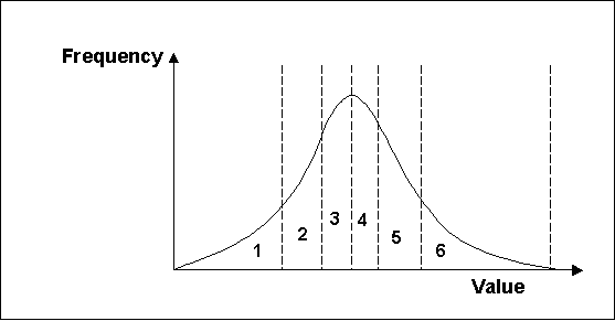
number of simulations, where n is the number of parameters and P is the number of segments for the ith parameter. For example, if there were three | number of simulations, where n is the number of parameters and P is the number of segments for the ith parameter. For example, if there were three parameters with four, four and five segments, the number of model runs would be as follows: | ||
<!--[[Image:comb_example.gif]]--> | <!--[[Image:comb_example.gif]]--> | ||


