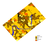
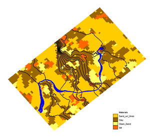
GMS includes an interface to the T-PROGS software developed by Steven Carle. The T-PROGS software is used to perform transition probability geostatistics on borehole data. The output of the T-PROGS software is a set of N material sets on a 3D grid. Each of the material sets is conditioned to the borehole data and the materials proportions and transitions between the boreholes follows the trends observed in the borehole data. These material sets can be used for stochastic simulations with MODFLOW. A sample material set generated by the TPROGS software is shown below. The T-PROGS software can also be used to generate multiple input data sets for the HUF package.
T-PROGS Interface
MODFLOW solution for a T-PROGS grid. Black lines are head contours and blue lines are pathlines for an extraction well.
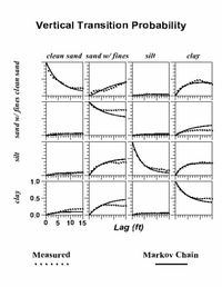
Observed transition probabilities (circles) and Markov chain model (solid lines) for a set of borehole data with four materials.
The T-PROGS software utilizes a transition probability-based geostatistical approach to model spatial variability by 3-D Markov Chains, set up indicator cokriging equations, and formulate the objective function for simulated annealing. The transition probability approach has several advantages over traditional indicator kriging methods. First, the transition probability approach considers asymmetric juxtapositional tendencies, such as fining-upwards sequences. Second, the transition probability approach has a conceptual framework for incorporating geologic interpretations into the development of cross-correlated spatial variability. Furthermore, the transition probability approach does not exclusively rely on empirical curve fitting to develop the indicator (cross-) variogram model. This is advantageous because geologic data are typically only adequate to develop a model of spatial variability in the vertical direction. The transition probability approach provides a conceptual framework to geologic insight into a simple and compact mathematical model, the Markov chain. This is accomplished by linking fundamental observable attributes – mean lengths, material proportions, anisotropy, and juxtapositioning – with Markov chain model parameters.
The first step in using T-PROGS is to import a set of borehole data. The borehole data are then passed to a utility within T-PROGS called GAMEAS that computes a set of transition probability curves as a function of lag distance for each category for a given sampling interval. A sample set of measured transition probability curves are shown by the dashed lines in the following figure.
Each curve represents the transition probability from material j to material k. The transition probability tjk(h) is defined by:

where x is a spatial location, h is the lag (separation vector), and j,k denote materials. Note that the curves on the diagonal represent auto-transition probabilities, and the curves on the off-diagonal represent cross-transition probabilities.
The next step in the analysis is to develop a Markov Chain model for the vertical direction that fits the observed vertical transition probability data. The Markov Chain curves are shown as solid lines in the preceeding figure. Mathematically, a Markov chain model applied to one-dimensional categorical data in a direction Φ assumes a matrix exponential form:

where h denotes a lag in the direction Φ, and RΦ denotes a transition rate matrix
File:Rate matrix.gif
with entries rjk,f representing the rate of change from category j to category k (conditional to the presence of j) per unit length in the direction Φ. The transition rates are adjusted to ensure a good fit between the Markov Chain model and the observed transition probability data.
Once the Markov chain is developed for the z direction from the borehole data, a model of spatial variability must be developed for the x and y directions. Borehole data are typically not sufficiently dense in these directions. However, the x and y-direction Markov chains can be developed by assuming that the juxtapositional tendencies and the proportions observed in the vertical direction also hold true in the horizontal directions. The modeler then provides an estimate of the ratio of the mean lengths in the x and y directions relative to the z direction, and the transition rate matrices for the x and y directions can be formulated. The x, y, and z Markov chains are converted into a continuous 3D Markov chain using the MCMOD utility within T-PROGS.
In the final phase of setting up a transition probability analysis using T-PROGS, the modeler creates a grid, specifies the number of model instances (N), and launches the TSIM utility. The TSIM code uses the 3D Markov chain to formulate both indicator cokriging equations and an objective function for simulated annealing. It generates stochastic simulations using a combination of modified versions of the GSLIB codes SISIM and ANNEAL.
T-PROGS OPTIONS
T-PROGS Options dialog with and without borehole data.
When a user selects the New Simulation command to initialize a T-PROGS simulation, the T-PROGS Options dialog appears. If boreholes do not exist in the model, an unconditioned simulation will be generated. In this case, the user selects the materials to be used and a corresponding background material. The Materials Editor button enables users to quickly create, delete, or rename materials and the material list is automatically regenerated. The upper part of the dialog lists the materials in the boreholes. The first column of toggles indicates which materials are to be used in the analysis. By default, all materials associated with the boreholes are selected. These toggles are necessary since it is possible that there may be materials defined in the materials list that are not associated with boreholes. The second column in the top section of the dialog lists the background material. By default, the material type that had the predominant occurrence in the boreholes (greatest proportion) is marked as the background material. When defining the transition probability data in the next section, the input parameters do not need to be edited for the background material. The parameters for this material are automatically adjusted to balance the equations.
Background Material
Application of the transition probability approach involves the designation of a background material. The probabilistic constraints of the Markov chains make it unnecessary to quantify data for one category. Not only is it unnecessary, but it is futile to do so because values will be overwritten in order to satisfy constraints. Conceptually, the background material can be described as the material that “fills” in the remaining areas not occupied by other units. For example, in a fluvial depositional system, a floodplain unit would tend to occupy area not filled with higher-energy depositional units and would therefore be a logical choice for the background material.
Azimuth
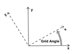
Azimuths for T-PROGS and 3D Grid.
The user also enters an azimuth in this dialog. The azimuth determines the orientation of the primary directions of the depositional trends in the strike/dip directions. These trends generally are aligned with the primary directions of horizontal flow in the aquifer. Theoretically, the azimuth can be oriented independently from the grid orientation. However, in practice, if the grid and azimuth orientations are offset by more than about 40 degrees, checkerboard patterns appear in the indicator array results. Hence, the azimuth orientation is set equal to the grid orientation by default. However, the grid angle is defined counterclockwise, and the azimuth angle is clockwise. Therefore, if the grid angle is 40 degrees, then the azimuth angle will be –40 degrees by default. If there is anisotropy in the xy plane, the azimuth angle should be set to the principle direction of the anisotropy. If anisotropy is not present, this angle should be coincident with the x-axis (the rows or j-direction) of the grid.
Material Limit
One limitation for both the cases with and without boreholes is that a maximum of nine materials (starting at GMS version 8.0 - five prior to 8.0) can be used in the T-PROGS algorithm. This limitation was imposed to keep the data processing and user-interface reasonably simple. Although nine materials present a limitation, borehole data can generally be easily condensed down to nine or fewer materials. Furthermore since this is a stochastic approach, which is based on probability, the detail generated with numerous materials is rarely justifiable anyway. In addition, as the number of materials increase, the ratio of process time to detail becomes inefficient.
Generating Material Sets with T-PROGS
The underlying equations solved by the T-PROGS software require an orthogonal grid with constant cell dimensions (X, Y, and Z). The delta X values can be different from the delta Y and delta Z values, and the delta Y values can be different from the delta Z values, but all cells must have the same change in X, Y, and Z dimensions. The MODFLOW model is capable of using the Layer Property Flow (LPF) Package with the Material ID option for assigning aquifer properties. With this option, each cell in the grid is assigned a material id and the aquifer properties (Kh, Kv, etc.) associated with each material are automatically assigned to the layer data arrays for the LPF package when the MODFLOW files are saved. The T-PROGS software generates multiple material sets (arrays of material ids), each of which represents a different realization of the aquifer heterogeneity. When running a MODFLOW simulation in stochastic mode, GMS automatically loads each of the N material sets generated by the T-PROGS software and saves N different sets of MODFLOW input files. The N solutions resulting from these simulations can be read into GMS and used to perform risk analyses such as probabilistic capture zone delineation.
One-Layer MODFLOW Grids

Sample material set generated by the T-PROGS software. Blue lines represent particle path lines and black lines are head contours.
Although MODFLOW is a three-dimensional model, a majority of the MODFLOW models constructed by typical users are 2D models consisting of one model layer. There are several reasons why 2D models are so common. One reason is that many of these models are regional models where the aquifer thickness is very small compared to the lateral extent of the model. As a result, the flow directions are primarily horizontal and little improvement is gained by adding multiple layers to the model. Even with local scale models, the aquifer thickness is often small enough that one-layer models are considered adequate. 2D models are also attractive due to the simplicity of the model increased computational efficiency. One of the problems associated with using multiple layers for MODFLOW models with unconfined aquifers is that as the water table fluctuates, the upper cells may go dry. These cells will not rewet even if the water table subsequently rises, unless the rewetting option has been selected in the flow package (BCF, LPF, or HUF). The rewetting issues can often be avoided with a one-layer model.
When developing a one-layer model, the modeler must determine how to distribute the hydraulic conductivity values within the layer. One option is to assume a homogenous aquifer; this is typically a gross over-simplification since aquifers are usually highly heterogeneous. Therefore, a common approach is to delineate zones of hydraulic conductivity by examining the subsurface stratigraphic data. In many cases, these data are in the form of borehole logs. These borehole logs often exhibit substantial heterogeneity and don’t always exhibit definitive trends between adjacent boreholes. Furthermore, the boreholes are often clustered with large regions of the model lacking any borehole data. The modeler then faces a difficult task of trying to determine a rational approach to delineating two-dimensional zones of hydraulic conductivity based on complex 3D borehole data.
As part of this research, we developed a technique for developing 2D zones of hydraulic conductivity from borehole logs using transition probability geostatistics. The technique is simple, fast, and preserves proportions and trends exhibited by the borehole data. The algorithm parses through each borehole and computes a predominant material at each borehole. When T-PROGS runs, the predominant material for each borehole is assigned to its corresponding location in the one-layer grid, and during the quenching process, simulations are conditioned to those data points.
Generating HUF Data with T-PROGS
Using transition probability geostatistics with MODFLOW models results in two basic limitations. First, the underlying stochastic algorithms used by the T-PROGS software are formulated such that the MODFLOW grid must have uniform row, column, and layer widths. The row width can be different from the column width, but each row must have the same width. This results in a uniform orthogonal grid. While MODFLOW grids are orthogonal in x and y, the layer thickness is allowed to vary on a cell-by-cell basis. This makes it possible for the layer boundaries to accurately model the ground surface and the tops and bottoms of aquifer units. If a purely orthogonal grid is used, irregular internal and external layer boundaries must be simulated in a stair-step fashion either by varying material properties or by activating/inactivating cells via the IBOUND array. A second limitation is that in order to get a high level of detail in the simulated heterogeneity, the grid cell dimensions are generally kept quite small. This can result in difficulties in the vertical dimension. The large number of layers with small layer thicknesses near the top of the model generally ensures that many of the cells in this region will be at or above the computed water table elevation (for simulations involving unconfined aquifers). As a result, these cells will undergo many of the numerical instabilities and increased computational effort issues associated with cell wetting and drying.
File:Huf sample.gif Sample HUF stratigraphy data generated by the T-PROGS software. Blue lines represent particle path lines and water table.
The Hydrogeologic Unit Flow (HUF) package released with MODFLOW 2000 makes it possible to overcome both of these limitations resulting in a powerful mechanism for incorporating transition probability geostatistics in MODFLOW simulations. With the HUF package, the modeler is allowed to input the vertical component of the stratigraphy in a grid-independent fashion. The stratigraphy data are defined using a set of elevation and thickness arrays. The first array defines the top elevation of the model. The remaining arrays define the thicknesses of a series of hydrogeologic units, starting at the top and progressing to the bottom of the model. For each array of thicknesses, many of the entries in the array may be zero. This makes it possible to simulate complex heterogeneity, including pinchouts and embedded lenses that would be difficult to simulate with the LPF and BCF packages.
The T-PROGS interface in GMS includes an option for integrating transition probability geostatistics results with the HUF package. The basic approach used by the option is to overlay a dense background grid on the MODFLOW grid and run T-PROGS on the background grid. A set of HUF arrays is then extracted from the background grid for use with the MODFLOW model. To use this option, user should first create a MODFLOW grid with the desired number of layers and the layer elevations should be interpolated to match the aquifer boundaries. The row and column widths are uniform but the layer thicknesses may vary from cell to cell. Then, when TSIM is launched, the HUF option should be selected. GMS then generates a background grid that encompasses the MODFLOW grid. The rows and columns of this grid match the MODFLOW grid but the layer thicknesses are uniform and relatively thin, resulting in a much greater number of layers than the MODFLOW grid. The user specifies the number of layers in this background grid. A T-PROGS simulation is then performed to get a set of material sets on the background grid. Each of the material sets in the T-PROGS output is then transferred from the background grid to a set of HUF elevation/thickness arrays. The HUF top elevation array is set equal to the top of the MODFLOW grid. The thickness arrays are then found by searching through the background grid to find the bottom elevations of contiguous groups of indicators. The elevations from these groups are then added to an appropriate elevation array in the HUF input. The resulting set of HUF input arrays are listed in GMS Project Explorer. By clicking on each item in the Project Explorer, the selected set of HUF arrays are loaded into the HUF package and the corresponding stratigraphy is displayed in the GMS window. The multiple HUF input arrays can be used to perform a stochastic simulation.
Notes
- ^
Carle, Steven F. (1999), T-PROGS: Transition Probability Geostatistical Software. Version 2.1, Davis, California, p. 6, http://gmsdocs.aquaveo.com/t-progs.pdf
- ^
Carle, Steven F. (1999), T-PROGS: Transition Probability Geostatistical Software. Version 2.1, Davis, California, p. 26, http://gmsdocs.aquaveo.com/t-progs.pdf
