GMS:Plot Wizard
Plots are useful for many purposes, such as extracting data from two or three dimensional objects and model verification. Plots are created through the Plot Wizard.
The Plot Wizard (Display | Plot Wizard) is used to create 2D plots. The Plot Wizard is composed of two steps described below. In addition, the types of plots that can be created are described and illustrated below.
Contents
- 1 Plot Wizard Step 1
- 2 Plot Wizard Step 2
- 2.1 Computed vs. Observed
- 2.2 Computed vs. Observed (Weighted)
- 2.3 Residual vs. Observed
- 2.4 Residual vs. Observed (Weighted)
- 2.5 Parameter Sensitivity
- 2.6 Error vs. Simulation
- 2.7 Error vs. Time Step
- 2.8 Error Summary
- 2.9 Time Series
- 2.10 Active Dataset Time Series
- 2.11 S/S Flow vs. Time
- 2.12 Mass vs. Time
- 2.13 Flow Budget vs. Time - 3D Grid or UGrid
- 2.14 Gage Package Value vs. Time
- 2.15 Finish
- 3 Right-Click Menu Commands
- 4 See also
Plot Wizard Step 1
In the first step, the plot type is selected. The types include:
- Computed vs. Observed Data
- Computed vs. Observed Data (Weighted)
- Residual vs. Observed Data
- Residual vs. Observed Data (Weighted)
- Parameter Sensitivities
- Error vs. Simulation
- Error vs. Time Step
- Error Summary
- Time Series
- Active Dataset Time Series Plot
- S/S Flow vs. Time
- Mass vs. Time
- Flow Budget vs. Time – 3D Grid
- Flow Budget vs. Time - UGrid
- Gage Package Value vs. Time
A sample and explanation are displayed for each plot type. The Next > button is undimmed if the necessary data for the selected plot type exists in the current project. This does not guarantee that GMS will create a plot. If the Next > button is disabled, a help text explaining the problem is displayed below the Plot Type box.
Plot Wizard Step 2
In the second step of the Plot Wizard, the attributes of each plot are set. The attributes associated with each plot type are explained below and can be located quickly by clicking on the desired plot type listed above. The options depend on the plot type and will be described below.
Computed vs. Observed
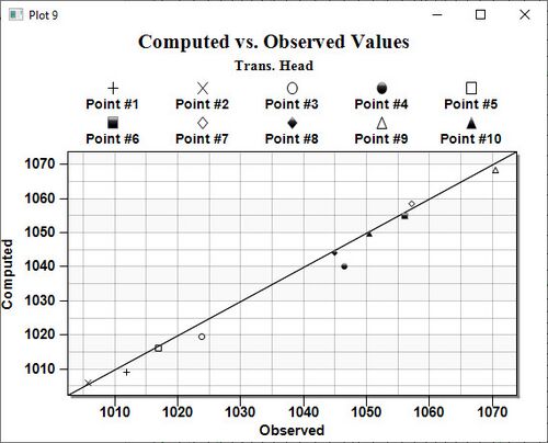
A Computed vs. Observed plot is used to display how well the entire set of observed values match a model solution. A 45° line is drawn on this plot, which represents a perfect correspondence between observed data and solution values. One symbol is drawn for each observation point at the intersection of the observed and computed values for the point. This plot can show the trend of the solution values with regard to matching the observed data. Only those points whose value is specified as observed for the selected data type will be shown in the plot. These plots are created in the Plot Wizard by setting the Plot Type to "Computed vs. Observed Data".
Computed vs. Observed Plot Options
The second step contains the following options.
- Coverage and Measurements
- The observation coverage and measurements can be selected for each plot. If only one observation coverage and measurement exist these are used by default.
- Use current solution
- This option causes the plot to compare the observed values with the values of the current solution and time step for each observation point. When the active solution changes, the plot is recomputed and updated. If only one solution is in memory then this option is defaulted and is not visible in the dialog.
- Use selected solutions
- This option causes the plot to compare the observed values with the values of the specified solution for each observation point. Changing the active solution does not affect the plot.
Computed vs. Observed Troubleshooting
If a plot will not generate or does not display significant data, it's possible that the conditions for the plot have not been set up correctly. To get a meaningful plot, take the following into account:
- This plot requires an observation coverage with feature points included that have observation data from the field. If there is more than one observation coverage, ensure the correct observation coverage is selected on step 2 of the Plot Wizard.
- This plot requires a simulation with calculated data of the same type of data as the observation coverage (head, for example). If the simulation does not have solution datasets, then this plot will not have significant results.
- The dataset desired for visualization should be selected in the Project Explorer. If the active item in the Project Explorer is not a dataset that can be plotted, then the plot may not display any information even if viable datasets are present in the project.
Computed vs. Observed (Weighted)
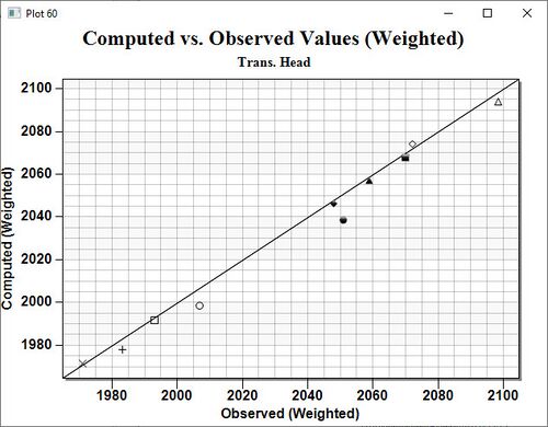
A Computed vs. Observed Weighted plot is used to display how well the entire set of weighted observed values match a model solution. These weights are set by selecting the Observation item in the MODFLOW menu. A 45° line is drawn on this plot, which represents a perfect correspondence between observed data and solution values. One symbol is drawn for each observation point at the intersection of the weighted observed and computed values for the point. This plot can show the trend of the solution values with regard to matching the weighted observed data. Only those points whose value is specified as observed for the selected data type will be shown in the plot. This plot is not available with transient data. These plots are created in the Plot Wizard by setting the Plot Type to "Computed vs. Observed Data (Weighted)".
Computed vs. Observed Weighted Plot Options
After the plot type is set in the first page of the Plot Wizard, the Next > button is clicked to open the Step 2 of 2 page For this plot, this page contains the following:
- Coverage and Measurements
- The observation coverage and measurements can be selected for each plot. If only one observation coverage and measurement exist these are used by default.
- Use current solution
- This option causes the plot to compare the weighted observed values with the values of the current solution and time step for each observation point. When the active solution changes, the plot is recomputed and updated. If only one solution is in memory then this option is defaulted and is not visible in the dialog.
- Use selected solutions
- This option causes the plot to compare the weighted observed values with the values of the specified solution for each observation point. Changing the active solution does not affect the plot.
Computed vs. Observed Plot (Weighted) Troubleshooting
If a plot will not generate or does not display significant data, it's possible that the conditions for the plot have not been set up correctly. To get a meaningful plot, take the following into account:
- This plot requires an observation coverage with feature points included that have observation data from the field. If there is more than one observation coverage, ensure the correct observation coverage is selected on step 2 of the Plot Wizard.
- This plot requires a simulation with calculated data of the same type of data as the observation coverage (head, for example). If the simulation does not have solution datasets, then this plot will not have significant results.
- The dataset desired for visualization should be selected in the Project Explorer. If the active item in the Project Explorer is not a dataset that can be plotted, then the plot may not display any information even if viable datasets are present in the project.
Residual vs. Observed
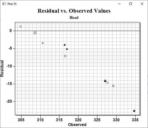
A Residual vs. Observed plot is used to display how well the entire set of observed values match a model solution. On this plot is drawn a horizontal line along an error of zero, representing what would be a perfect correspondence between observed data and solution values. Then, one symbol is drawn for each observation point at the intersection of the observed and residual (computed minus observed) values for the point. This plot can show the trend of the solution values with regards to matching the observed data. Only those points whose value is specified as observed for the selected data type will appear in the plot. These plots are created in the Plot Wizard by setting the Plot Type to "Residual vs. Observed Data".
Residual vs. Observed Plot Options
After the plot type is set in the first page of the Plot Wizard, the Next > button is clicked to open the Page 2 of 2 wizard page. This page contains the following:
- Coverage and Measurements
- The observation coverage and measurements can be selected for each plot. If only one observation coverage and measurement exist these are used by default.
- Use current solution
- This option causes the plot to compare the observed values with the residual values of the current solution and time step for each observation point. When the active solution changes, the plot is recomputed and updated. If only one solution is in memory then this option is defaulted and is not visible in the dialog.
- Use selected solutions
- This option causes the plot to compare the observed values with the residual values of the specified solution for each observation point. Changing the active solution does not affect the plot.
Residual vs. Observed Troubleshooting
If a plot will not generate or does not display significant data, it's possible that the conditions for the plot have not been set up correctly. To get a meaningful plot, take the following into account:
- This plot requires an observation coverage with feature points included that have observation data from the field. If there is more than one observation coverage, ensure the correct observation coverage is selected on step 2 of the Plot Wizard.
- This plot requires a simulation with calculated data of the same type of data as the observation coverage (head, for example). If the simulation does not have solution datasets, then this plot will not have significant results.
- The dataset desired for visualization should be selected in the Project Explorer. If the active item in the Project Explorer is not a dataset that can be plotted, then the plot may not display any information even if viable datasets are present in the project.
Residual vs. Observed (Weighted)
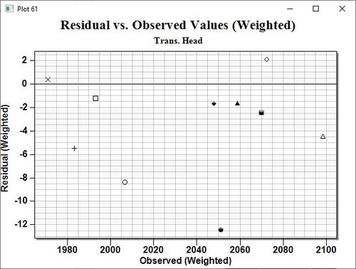
A Residual vs. Observed (Weighted) plot is used to display how well the entire set of weighted observed values match a model solution. On this plot is drawn a horizontal line along an error of zero, representing what would be a perfect correspondence between weighted observed data and solution values. One symbol is drawn for each observation point at the intersection of the weighted observed and residual (computed minus observed) values for the point. This plot can show the trend of the solution values with regards to matching the weighted observed data. Only those points whose value is specified as observed for the selected data type will be shown in the plot. This plot is not available with transient data. These plots are created in the Plot Wizard by setting the Plot Type to "Residual vs. Observed Data (Weighted)".
Residual vs. Observed Weighted Plot Options
After the plot type is set in the first page of the Plot Wizard, the Next > button is clicked to open the Page 2 of 2 wizard page. This page contains the following:
- Coverage and Measurements
- The observation coverage and measurements can be selected for each plot. If only one observation coverage and measurement exist these are used by default.
- Use current solution
- This option causes the plot to compare the weighted observed values with the residual values of the current solution and time step for each observation point. When the active solution changes, the plot is recomputed and updated. If only one solution is in memory then this option is defaulted and is not visible in the dialog.
- Use selected solutions
- This option causes the plot to compare the weighted observed values with the residual values of the specified solution for each observation point. Changing the active solution does not affect the plot.
Residual vs. Observed (Weighted) Troubleshooting
If a plot will not generate or does not display significant data, it's possible that the conditions for the plot have not been set up correctly. To get a meaningful plot, take the following into account:
- This plot requires an observation coverage with feature points included that have observation data from the field. If there is more than one observation coverage, ensure the correct observation coverage is selected on step 2 of the Plot Wizard.
- This plot requires a simulation with calculated data of the same type of data as the observation coverage (head, for example). If the simulation does not have solution datasets, then this plot will not have significant results.
- The dataset desired for visualization should be selected in the Project Explorer. If the active item in the Project Explorer is not a dataset that can be plotted, then the plot may not display any information even if viable datasets are present in the project.
Parameter Sensitivity
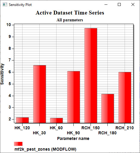
A Parameter Sensitivity plot is used to display the sensitivity of the MODFLOW parameters. These plots are created in the Plot Wizard by setting the Plot Type to "Parameter Sensitivities".
Parameter Sensitivity Plot Options
After the plot type is set in the first page of the Plot Wizard, the Next > button is clicked to open the Page 2 of 2 wizard page. This page contains the following:
- Parameter Type
- This option changes the parameter type displayed.
- Use current solution
- This option causes the plot to compare parameter sensitivities of the current solution. When the active solution changes, the plot is recomputed and updated. If only one solution is in memory then this option is defaulted and is not visible in the dialog.
- Use selected solutions
- This option causes the plot to compare parameter sensitivities of the specified solution. Changing the active solution does not affect the plot.
Parameter Sensitivity Plot Troubleshooting
If a plot will not generate or does not display significant data, it's possible that the conditions for the plot have not been set up correctly. To get a meaningful plot, take the following into account:
- This plot requires an observation coverage with feature points included that have observation data from the field.
- This plot requires sensitivity data calculated as part of a MODFLOW simulation.
- Selecting the correct dataset in the Project Explorer is essential to visualizing the results. If there is sensitivity data in the project, but the plot is not representing it, try selecting different solution datasets in the Project Explorer. The Sensitivity Plot display updates with each new selection, so it will become obvious which dataset must be active for the plot to accurately represent the data. Selecting the items under the Parameters folder in the Project Explorer does not draw the data in the plot.
Error vs. Simulation
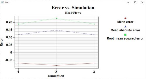
An Error vs. Simulation plot is generally used with steady-state simulations and measurement types. It may be used in transient simulations. This plot can display the mean error, mean absolute error, and root mean squared error between successive solutions and observed data. Various simulations would be run after changing model parameters, such as hydraulic conductivity or recharge. The plot will show trends in the solution to see if model parameter changes are causing better calibration with measured field data. Error vs. Simulation plots are created in the Plot Wizard by setting the Plot Type to "Error vs. Simulation".
Error vs. Simulation Plot Options
After the plot type is set in the First Page of the Plot Wizard, the Next > button is clicked to open the Page 2 of 2 wizard page. This page contains the following:
- Solutions
- This lists all available solutions.
- Move Up/Move Down
- GMS initially shows the solutions in the order they were opened. However, this is not necessarily the order in which they were run. To change the order, highlight a solution and move it up or down to rearrange their order.
- Check Box Options
- There are three options that can be turned on or off. They determine whether the mean error, mean absolute error, and root mean squared error plots should be shown. Because these values are an average of all observation points, their line and symbol styles are not linked to any one observation point, but can be defined by clicking on the appropriate canvas window in the dialog.
Error vs. Simulation Troubleshooting
If a plot will not generate or does not display significant data, it's possible that the conditions for the plot have not been set up correctly. To get a meaningful plot, take the following into account:
- This plot requires data from multiple simulation runs for comparing to each other.
- This data can be put in one project by using the Save As function to save the project with a new name before each MODFLOW simulation run. If the project isn't saved with a new name before each simulation run, the program will overwrite the former simulation results and the Error vs. Simulation plot will not have the desired comparison between simulation results.
- This plot requires an observation coverage with feature points that include data from the field. This data is used to judge the accuracy of the each simulation run. If there is more than one observation coverage, ensure the correct observation coverage is selected on step 2 of the Plot Wizard.
- It's possible that the wrong geometry is active. Since simulation solutions are usually attached to geometries, it's important to select the geometry with the solutions to be compared.
Error vs. Time Step
An Error vs. Time Step plot is used with transient simulations to display the mean error, mean absolute error, and root mean squared error between a solution and observed data as a function of time. This plot applies to a single dataset in a model solution. Transient measurement types will show the average errors at each time step of the dataset. Error vs. Time Step plots are created in the Plot Wizard by setting the Plot Type to "Error vs. Time Step". A sample plot is shown in the figure.
Beginning with version 8.0, this plot can no longer be used with MODFLOW.
Error vs. Time Step Plot Options
After the plot type is set in the first page of the Plot Wizard, the Next > button is clicked to open the Page 2 of 2 wizard page. This page contains the following:
- Use current solution
- This option causes the plot to display the error relative to the time step of the current solution. When the active solution changes, the plot is recomputed and updated. If only one solution is in memory then this option is defaulted.
- Use selected solutions
- This option causes the plot to display the error relative to the time step of the specified solution. Changing the active solution does not affect the plot.
- Observed
- This lists all available measurement types that were set up in the Observation Coverage Options dialog, both constant and transient. A constant measurement should be used for solutions with only one time step, while a transient measurement should be used for transient solutions. Select the measurement type in the combo box that is being compared. If only one exists then it is used by default.
- Check Box Options
- There are three options that can be turned on or off. They determine whether the mean error, mean absolute error, and root mean squared error plots should be shown. Because these values are an average of all observation points, their line and symbol styles are not linked to any one observation point, but can be defined by clicking on the appropriate canvas window in the dialog.
Error vs. Time Step Troubleshooting
If a plot will not generate or does not display significant data, it's possible that the conditions for the plot have not been set up correctly. To get a meaningful plot, take the following into account:
- As noted above, this plot type cannot be used with MODFLOW beginning with version 8.0 of GMS. Ensure that the data to be visualized is not MODFLOW data.
- This plot requires an observation coverage to compute error. Errors in the computed values are calculated based on observed values defined in an observation coverage. If there is more than one observation coverage, ensure the correct observation coverage is selected on step 2 of the Plot Wizard.
- This plot requires a transient dataset to plot error against time.
- Selecting the correct geometry/dataset is important for this plot. If significant results are not displaying, select the desired dataset in the Project Explorer. If it's unclear how to get the desired dataset to display, select different items in the Project Explorer until it's clear the desired dataset is active.
Error Summary
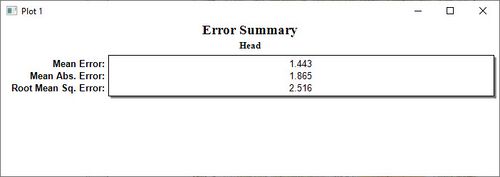
See the Error Summary Plot page for more details. An error summary plot is used to display the mean error, mean absolute error, and root mean squared error for a solution. Error summary plots are created in the Plot Wizard by setting the Plot Type to "Error Summary".
Beginning with version 8.0, this plot can no longer be used with MODFLOW. This information can be found by right-clicking on the MODFLOW solution in the Project Explorer and selecting Properties.
Error Summary Plot Options
After the plot type is set in the first page of the Plot Wizard, the Next > button is clicked to open the Page 2 of 2 wizard page. This page contains the following:
- Use active solution
- This option causes the plot to show a summary of mean error between the set of observed values with the values of the active solution for each observation point. When the active solution changes, the plot is recomputed and updated. This option is on by default at this time.
- All time steps
- This option shows the mean error for all time steps instead of only at the current or specified time step value.
Error Summary Troubleshooting
If a plot will not generate or does not display significant data, it's possible that the conditions for the plot have not been set up correctly. To get a meaningful plot, take the following into account:
- As noted above, this plot type cannot be used with MODFLOW beginning with version 8.0 of GMS. Ensure that the data to be visualized is not MODFLOW data.
- This plot requires an observation coverage to compute error. Errors in the computed values are calculated based on observed values defined in an observation coverage. If there is more than one observation coverage, ensure the correct observation coverage is selected on step 2 of the Plot Wizard.
Time Series
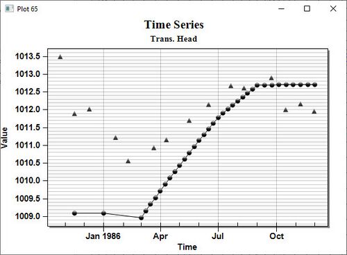
A time series plot is used to display the time variation of one or more scalar datasets associated with a given point inside a model solution. In addition, if transient calibration data has been defined, the plot can show time variant calibration targets. Only transient datasets may be used in these plots. Time series plots are created in the Plot Wizard by setting the Plot Type to "Time Series". A sample plot is shown in the figure.
Beginning with version 8.0, these plots have been changed to show observation targets instead of a "band" around the observed data.
Time Series Plot Options
After the plot type is set in the first page of the Plot Wizard, the Next > button is clicked to open the Page 2 of 2 wizard page. This page contains the following:
- Coverage and Measurements
- The observation coverage and measurements can be selected for each plot. If only one observation coverage and measurement exist these are used by default. All measurements can also be selected to plot all of the different measurements on one plot.
- Use current solution
- This option causes the plot to display the values of the active solution for each observation point being plotted. When the active solution changes, the plot is recomputed and updated. If only one solution is in memory then this option is defaulted.
- Use selected solutions
- This option causes the plot to display the values of one or more specified solutions for each point being plotted. Changing the active solution does not affect the plot.
- Selected Points
- Each of the observation points are shown in a spreadsheet. The box in the show column determines which observation points will be displayed in a time series plot in the Plot Window. This way, only certain points are plotted in each individual time series plot. All the points can either be turned on or off by selecting the corresponding buttons below the spreadsheet.
- Calibration Target
- Turn this on to display observation targets in the plot.
- Time interval
- A starting time and an ending time of observations can be specified by the combo boxes. Only the interval chosen will be shown on the time series plot.
Time Series Troubleshooting
If a plot will not generate or does not display significant data, it's possible that the conditions for the plot have not been set up correctly. To get a meaningful plot, take the following into account:
- This plot requires an observation coverage with feature points included that have observation data from the field. If there is more than one observation coverage, ensure the correct observation coverage is selected on step 2 of the Plot Wizard.
- A point from the observation coverage must be selected. This point can be selected in the Graphics Window or in the spreadsheet on the second page of the Plot Wizard. If a point is not selected, the plot will not have significant results.
- This plot requires a simulation with calculated transient data of the same type of data as the observation coverage (head, for example). If the simulation has not been run, then this plot will not have significant results.
Active Dataset Time Series
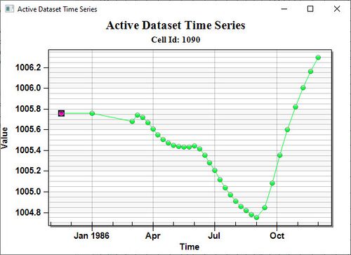
An Active Dataset Time Series plot is used to display the time variation of one or more scalar datasets associated to a given geometric element selected in a model solution. Active Dataset Time Series plots are created in the Plot Wizard by setting the Plot Type to "Active Dataset Time Series".
Active Dataset Time Series Plot Options
After the plot type is set in the first page of the Plot Wizard, the Finish button is clicked to create the active dataset time series plot. For 2D and 3D grids select a grid cell and for 2D and 3D meshes select a node to display the scalar values of the dataset at that location over time. Select up to five locations to be plotted on one plot.
Active Dataset Time Series Troubleshooting
If a plot will not generate or does not display significant data, it's possible that the conditions for the plot have not been set up correctly. To get a meaningful plot, take the following into account:
- This plot needs a transient dataset interpolated to a mesh or a grid active in the Project Explorer and visible in the Graphics Window. This is usually a dataset associated with a model solution.
- A specific element of the geometry must be selected in order to generate meaningful data in this plot. Grids require that a grid cell be selected. Meshes require that a mesh node be selected.
S/S Flow vs. Time
An S/S Flow vs. Time plot is used to display the flow or water over time for a selected feature object or grid cell. Flow vs. Time plots are created in the Plot Wizard by setting the Plot Type to S/S Flow vs. Time.
S/S Flow vs. Time Plot Options
After the plot type is set in the first page of the Plot Wizard, click Next > to open the Step 2 of 2 wizard page. On this page these options are available:
- Calibration Target
- Observed Values
The Finish button is clicked to create the flow vs time plot. This plot will report the flow either by selecting a feature object defined as a MODFLOW source/sink in the map module. To change the plot options for the Flow vs. Time Plot, right-click on the plot and select the Plot Data command.
S/S Flow vs. Time Troubleshooting
If a plot will not generate or does not display significant data, it's possible that the conditions for the plot have not been set up correctly. To get a meaningful plot, take the following into account:
- This plot requires an arc labeled as a source/sink for MODFLOW. It must be selected in the Graphics Window for data to show in the plot.
- This plot requires a 3D Grid with simulation data that the selected feature object was used to help calculate.
- This plot requires an observation coverage with at least one observation point in it with relevant data.
Mass vs. Time
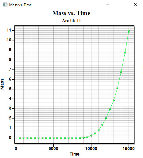
Mass vs. Time plots are created in the Plot Wizard by setting the Plot Type to Mass vs. Time.
Mass vs. Time Troubleshooting
If a plot will not generate or does not display significant data, it's possible that the conditions for the plot have not been set up correctly. To get a meaningful plot, take the following into account:
- This plot requires a feature object that has been assigned a source/sink type. The feature object must be run as part of a simulation that calculates data relevant to the plot. This feature object must be selected for data to show in the plot.
- This plot requires a 3D Grid and a simulation that has been run using the feature object whose data is to be plotted.
Flow Budget vs. Time - 3D Grid or UGrid
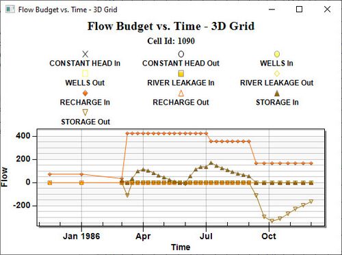
A Flow Budget vs. Time plot is used to display the flow or water over time for selected grid cell or for zone budget ids. Flow Budget vs. Time plots are created in the Plot Wizard by setting the Plot Type to "Flow Budget vs. Time - 3D Grid" or Flow Budget vs. Time – UGrid.
Flow Budget vs. Time Plot Options
After the plot type is set in the first page of the Plot Wizard, the Next > button is clicked to open the Page 2 of 2 wizard page. The options on this page are discussed below. The Finish button is clicked to create the flow budget vs. time plot. This plot will report the flow either by selecting a group of cells in the 3D grid or by using the zone budget ids.
- Display using
- This option allows users to determine the data to plot. The flow budget will be computed either from the selected 3D grid cells or from the selected zone budget ids in the spreadsheet.
- Sources/Sinks
- This spreadsheet allows users to select what source/sink flows to plot. The options are: Storage, Constant Head, Drains, General Heads, Rivers, Streams, Recharge, Evapotranspiration, and Total Source/Sink flow in and out of the cells.
Flow Budget vs. Time Troubleshooting
If a plot will not generate or does not display significant data, it's possible that the conditions for the plot have not been set up correctly. To get a meaningful plot, take the following into account:
- This plot requires a grid of the appropriate type (3D Grid or UGrid).
- This plot requires a coverage with the appropriate attributes selected in the Coverage Setup dialog.
- This plot requires a transient MODFLOW simulation attached to the geometry.
- The data displayed depends on the active solution in the Project Explorer. Make sure the desired dataset is active in the Project Explorer for visualization.
Gage Package Value vs. Time
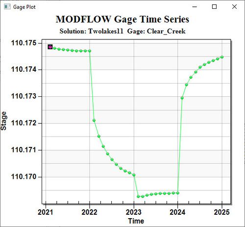
This plot shows a time series for a single gage package column. After the plot type is set in the first page of the Plot Wizard, the Next button is clicked to open the Gage Package Time Series wizard page. To generate a gage plot the gage file needs to be selected from the list on the left, and the data column from the list on the right. If GMS is unable to properly read the data from the gage file, an error is shown in the wizard page to the right of the data column list.
Gage Package Value vs. Time Troubleshooting
If a plot will not generate or does not display significant data, it's possible that the conditions for the plot have not been set up correctly. To get a meaningful plot, take the following into account:
- This plot requires a transient MODFLOW simulation with the GAGE package set up, so it generates GAGE files. For the plot to display, it is necessary to have GAGE files actually in the Project Explorer.
- This plot will not generate unless a dataset in the model solution is the active dataset in the Project Explorer. Select a dataset in the model solution to make this plot available. Selecting the Gage files themselves will not make the plot available.
Finish
When the Finish button is selected, a window is opened with the plot. Plot windows are created each time the Plot Wizard is run. See the 2D Plots discussion for information on editing plots that have been created.
Right-Click Menu Commands
Once the plot has been created, the appearance and data of the plot can be altered with commands accessed by right-clicking on the plot window. The commands available through the right-click menu are described below.
- Plot Data
- Brings up the second step of the Plot Wizard where the attributes of each plot are set. The plot data can be updated based upon the type of plot. For histogram plots it brings up a dialog used to edit the precision displayed on the plot.
- Display Options
- Allows changing general display attributes of the plot (border style, precision, axis type, fonts, colors, etc.).
- Axis Titles
- Used to change the x and y axis titles.
- Set As Display Defaults
- Saves the plots current settings as the default settings.
- Legend
- Submenu that allows selecting the legend location. The maximum number of points included in the legend depends upon the size of the plot window.
- Symbol Size
- Submenu that allows adjusting the size of the symbols in the plot.
- Frame Plot
- If the view is zoomed in to a portion of the plot, resets zoom extents.
- Maximize Plot
- Expands the plot to fit nearly full screen. Does not expand Plot dialog. Click in the upper-left corner or click the Esc key to exit the full screen view.
- View Values
- Brings up a spreadsheet containing the data points associated with the current plot.
- Export/Print
- Brings up a dialog showing options for printing or exporting the plots values.
See also
| GMS – Groundwater Modeling System | ||
|---|---|---|
| Modules: | 2D Grid • 2D Mesh • 2D Scatter Point • 3D Grid • 3D Mesh • 3D Scatter Point • Boreholes • GIS • Map • Solid • TINs • UGrids | |
| Models: | FEFLOW • FEMWATER • HydroGeoSphere • MODAEM • MODFLOW • MODPATH • mod-PATH3DU • MT3DMS • MT3D-USGS • PEST • PHT3D • RT3D • SEAM3D • SEAWAT • SEEP2D • T-PROGS • ZONEBUDGET | |
| Aquaveo | ||
