User:Rcorrigan/Edits Riley didn't finish
3D INTERPOLATION OPTIONS
3D scatter point sets are used for interpolation to other data types such as grids and meshes. Interpolation is useful for such tasks as isosurface rendering or setting up input data for a model. Since no interpolation scheme is superior in all cases, several interpolation techniques are provided in GMS.
The basic approach to performing an interpolation is to select an appropriate interpolation scheme and interpolation parameters, and then interpolate to the desired object using one of the interpolation commands (to 3D grid, to 3D mesh, etc.) described below.
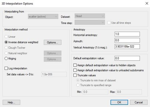
The interpolation options are selected using the 3D Interpolation Options dialog which is accessed through the Interpolation Options command in the Interpolation menu. The Interpolation menu appears when a scatter set item is active in the Project Explorer. Once a set of options is selected, those options are used for all subsequent interpolation commands. The options in the 3D Interpolation Options dialog are as follows:
Active Dataset
Interpolation is always performed using the active dataset of the active scatter point set. The active dataset is normally selected in the Project Explorer. The name of the current active dataset is listed at the top of the 3D Interpolation Options dialog in the Interpolating from section.
Object displays the name of the active 3D scatter item, and Dataset displays the name of the 3D scatter dataset.
If the active dataset is transient then more interpolation options are available.
Steady State vs. Transient Interpolation
If the active dataset happens to be a transient dataset, two options are available:
- Steady state interpolation can be performed using only the selected time step of the active dataset.
- Transient interpolation can be performed using all of the time steps.
By default, only the selected time step is used. The time step is shown next to Time step at the top of the dialog. All of the time steps can be selected by selecting the Use all time steps option next to the Time step box. If all time steps are chosen, GMS begins with the first time step in the list and repeatedly interpolates from the scatter point set to the target object, one time step at a time, for all of the time steps. As a result, a dataset is created on the target object with a set of time steps matching the time steps on the scatter point set.
When performing transient interpolation with the kriging option, special care should be taken with regard to the variogram. Since each time step represents a separate set of data, technically, a separate variogram (or set of variograms) should be created for each time step (GMS stores a separate variogram for each step). This can be accomplished by selecting each time step one at a time using the Time step combo box at the top of the Interpolation Options dialog, and creating a new variogram for each time step.
Interpolation Methods
The following methods are supported for 3D interpolation in GMS:
- Inverse Distance Weighted Interpolation – Based on the assumption that the interpolating surface should be influenced most by the nearby points and less by the more distant points.
- Kriging – Based on the assumption that the parameter being interpolated can be treated as a regionalized variable.
Log interpolation is also supported.
Anisotropy
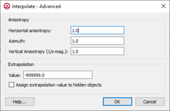
Sometimes the data associated with a scatter point set will have directional tendencies. The Azimuth and Horizontal Anisotropy allow taking into account these tendencies.
Vertical Anisotropy
In 3D, vertical anisotropy is also available. In previous versions of GMS it was possible to enter a Z scale. Vertical anisotropy is 1 over the Z scale. This notation was changed to be consistent with Kriging.
Occasionally, scatter point sets are sampled along vertical traces. In such cases, the distances between scatter points along the vertical traces are an order of magnitude smaller than the distances between scatter points along the horizontal plane. For example, if the scatter point set was obtained from borehole data, the distance between scatter points may be a few centimeters, whereas the distance between boreholes may be several meters. This disparity in scaling causes clustering and can be a source of poor results in some interpolation methods.
The effects of clustering along vertical traces can be minimized using the vertical anisotropy option in the 3D Interpolation Options dialog. The Z coordinate of each of the scatter points is multiplied by 1 divided by the vertical anisotropy parameter prior to interpolation. Thus, if the vertical anisotropy parameter is less than 1.0, scatter points along the same vertical axis appear farther apart than they really are and scatter points in the same horizontal plane appear closer than they really are. As a result, points in the same horizontal plane are given a higher relative weight than points along the Z axis. This can result in improved accuracy, especially in cases where the horizontal correlation between scatter points is expected to be greater than the vertical correlation (which is typically the case in soils since soils are deposited in horizontal layers).
Extrapolation
Although they are referred to as interpolation schemes, most of the schemes supported by GMS perform both interpolation and extrapolation. That is, they can estimate a value at points both inside and outside the scatter point set. Obviously, the interpolated values are more accurate than the extrapolated values. Nevertheless, it is often necessary to perform extrapolation. Some of the schemes, however, perform interpolation but cannot be used for extrapolation. Interpolation points outside the scatter set are assigned the Default extrapolation value.
This option will assign the default extrapolation value to all cells that are hidden using the Hide command in the Display | Visibility menu option (see Display Menu).
Truncation
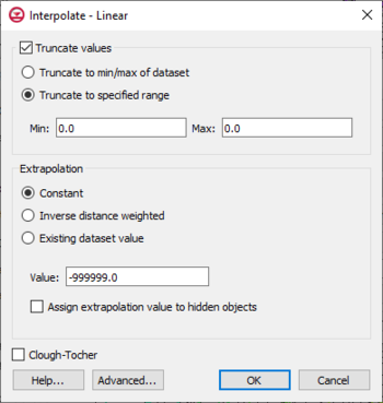
When interpolating a set of values, it is sometimes useful to limit the interpolated values to lie between a minimum and maximum value. For example, when interpolating contaminant concentrations, a negative value of concentration is meaningless. However, many interpolation schemes will produce negative values even if all of the scatter points have positive values. This occurs in areas where the trend in the data is toward a zero value. The interpolation may extend the trend beyond a zero value into the negative range. In such cases it is useful to limit the minimum interpolated value to zero. Interpolated values can be limited to a given range by selecting the Truncate values option in the 3D Interpolation Options dialog. The minimum and maximum values can either set according to the minimum and maximum of the dataset or according to specified range.
Related Topics
| [hide] GMS – Groundwater Modeling System | ||
|---|---|---|
| Modules: | 2D Grid • 2D Mesh • 2D Scatter Point • 3D Grid • 3D Mesh • 3D Scatter Point • Boreholes • GIS • Map • Solid • TINs • UGrids | |
| Models: | FEFLOW • FEMWATER • HydroGeoSphere • MODAEM • MODFLOW • MODPATH • mod-PATH3DU • MT3DMS • MT3D-USGS • PEST • PHT3D • RT3D • SEAM3D • SEAWAT • SEEP2D • T-PROGS • ZONEBUDGET | |
| Aquaveo | ||
UGRID INVERSE DISTANCE WEIGHTED INTERPOLATION
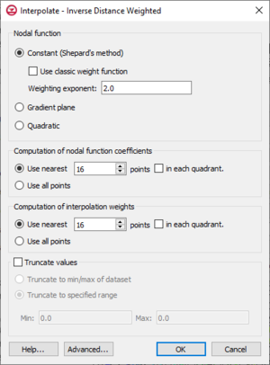
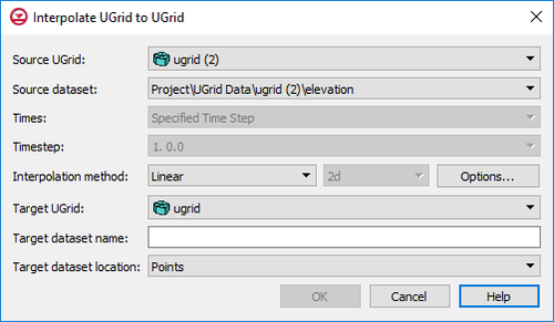
One of the most commonly used techniques for interpolation of point data is inverse distance weighted (IDW) interpolation. Inverse distance weighted methods are based on the assumption that the interpolating surface should be influenced most by the nearby points and less by the more distant points. The interpolated surface is a weighted average of the point data; the weight assigned to each point diminishes as the distance to the interpolation location increases. Several options are available for inverse distance weighted interpolation. The options are selected using the IDW Interpolation Options dialog. This dialog is accessed through the Options button next to the Inverse distance weighted item in the Interpolate UGrid to UGrid dialog.
The options in the dialog are as follows:
- Nodal function
- Constant (Shepard's Method) – The simplest form of inverse distance weighted interpolation. Includes the option to Use classic weight function to enter a Weighting exponent.
- Gradient Plane Nodal Functions – Variation of Shepard's method with nodal functions or individual functions defined at each point
- Quadratic Nodal Functions – Makes use of quadratic polynomials to constrain nodal functions.
- Computation of nodal function coefficients – Uses a subset of the data points. Using a subset of the data points drops distant points from consideration since they are unlikely to have a large influence on the nodal function. In addition, using a subset can speed up the computations since less points are involved. Two options are available for defining which points are included in the subset. In the first approach, only the nearest N points are used. In the second approach, only the nearest N points in each quadrant are used as illustrated in the figure below. The second approach may give better results if the data points tend to be clustered.
- Computation of interpolation weights – Uses a subset of the data points as with the Computation of nodal function coefficients section.
- Truncate values – This section allows for limiting the interpolated values to lie between the minimum and maximum value.
- Truncate to min/max of dataset – Limits the interpolated values to the minimum and maximum values in the original dataset.
- Truncate to specified range – Allows setting a user specified minimum and maximum value range.
- Min – Manually sets a minimum value.
- Max – Manually sets a maximum value.
- Advanced – This button will open the Interpolate – Advanced dialog where options for anisotropy and extrapolation can be adjusted.
Related Topics
| [hide] GMS – Groundwater Modeling System | ||
|---|---|---|
| Modules: | 2D Grid • 2D Mesh • 2D Scatter Point • 3D Grid • 3D Mesh • 3D Scatter Point • Boreholes • GIS • Map • Solid • TINs • UGrids | |
| Models: | FEFLOW • FEMWATER • HydroGeoSphere • MODAEM • MODFLOW • MODPATH • mod-PATH3DU • MT3DMS • MT3D-USGS • PEST • PHT3D • RT3D • SEAM3D • SEAWAT • SEEP2D • T-PROGS • ZONEBUDGET | |
| Aquaveo | ||
UGRID interpolation
