GMS:Stochastic Modeling: Difference between revisions
From XMS Wiki
Jump to navigationJump to search
No edit summary |
|||
| (3 intermediate revisions by the same user not shown) | |||
| Line 2: | Line 2: | ||
There are three methods in GMS for stochastic modeling using MODFLOW 2000 or 2005. The first, [[GMS:Stochastic Modeling#Using Parameter Zonation With Stochastic Modeling|parameter zonation]], uses either a [[GMS:Stochastic Modeling#Using Parameter Zonation With Stochastic Modeling|random sampling]], a [[GMS:Stochastic Modeling#Using Parameter Zonation With Stochastic Modeling|Latin hypercube sampling]], or [[GMS:Gaussian Field Generator|Gaussian fields]] to generate the different realizations. The second approach uses [[GMS:Stochastic Modeling#Using Indicator Simulations With Stochastic Modeling|indicator simulations]] generated by [[GMS:T-PROGS|T-PROGS]]. The third, the Null Space Monte Carlo (NSMC) method, generates multiple generated models with different sets of parameters (in GMS 9.0 and after). | There are three methods in GMS for stochastic modeling using MODFLOW 2000 or 2005. The first, [[GMS:Stochastic Modeling#Using Parameter Zonation With Stochastic Modeling|parameter zonation]], uses either a [[GMS:Stochastic Modeling#Using Parameter Zonation With Stochastic Modeling|random sampling]], a [[GMS:Stochastic Modeling#Using Parameter Zonation With Stochastic Modeling|Latin hypercube sampling]], or [[GMS:Gaussian Field Generator|Gaussian fields]] to generate the different realizations. The second approach uses [[GMS:Stochastic Modeling#Using Indicator Simulations With Stochastic Modeling|indicator simulations]] generated by [[GMS:T-PROGS|T-PROGS]]. The third, the Null Space Monte Carlo (NSMC) method, generates multiple generated models with different sets of parameters (in GMS 9.0 and after). | ||
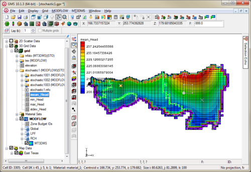
After the stochastic simulation results are generated, a user can view these results using the [[GMS:The GMS Window|Project Explorer]]. A user can also refine the results by using the [[GMS:Risk Analysis Wizard|''Risk Analysis Wizard'']] or [[GMS:Stochastic Modeling#Statistical Analysis of Stochastic MODFLOW/MT3D solutions| | After the stochastic simulation results are generated, a user can view these results using the [[GMS:The GMS Window|Project Explorer]]. A user can also refine the results by using the [[GMS:Risk Analysis Wizard|''Risk Analysis Wizard'']] or [[GMS:Stochastic Modeling#Statistical Analysis of Stochastic MODFLOW/MT3D solutions|statistical analysis of stochastic solutions]]. | ||
The stochastic modeling options can be added to a [http://www.aquaveo.com/software/gms-pricing paid edition] of GMS. | The stochastic modeling options can be added to a [http://www.aquaveo.com/software/gms-pricing paid edition] of GMS. | ||
| Line 71: | Line 71: | ||
<!--<math>f(x) = \dfrac{1}{\sqrt{2 \pi \sigma}} \text{exp} \left ( - \frac{(x-u)^2}{2 \sigma ^2} \right )</math>--> | <!--<math>f(x) = \dfrac{1}{\sqrt{2 \pi \sigma}} \text{exp} \left ( - \frac{(x-u)^2}{2 \sigma ^2} \right )</math>--> | ||
[[Image:stochasticeq1.jpg]] | :[[Image:stochasticeq1.jpg]] | ||
where σ is the standard deviation, μ is the mean, and x is the value being sampled. A uniform distribution can be defined as: | where σ is the standard deviation, μ is the mean, and x is the value being sampled. A uniform distribution can be defined as: | ||
<!--<math>f(x) = \dfrac{1}{\beta - \alpha}</math>--> | <!--<math>f(x) = \dfrac{1}{\beta - \alpha}</math>--> | ||
[[Image:stochasticeq2.jpg]] | :[[Image:stochasticeq2.jpg]] | ||
where α and β are the bounds of the parameter value x. | where α and β are the bounds of the parameter value x. | ||
| Line 93: | Line 93: | ||
<!--<math>\prod_{i=1}^n P_i</math>--> | <!--<math>\prod_{i=1}^n P_i</math>--> | ||
[[Image:stochasticeq3.jpg]] | :[[Image:stochasticeq3.jpg]] | ||
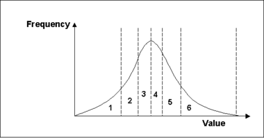
number of simulations, where n is the number of parameters and P is the number of segments for the ith parameter. For example, if there were three parameters with four, four, and five segments, the number of model runs would be as follows: | number of simulations, where n is the number of parameters and P is the number of segments for the ith parameter. For example, if there were three parameters with four, four, and five segments, the number of model runs would be as follows: | ||
<!--<math>\ 4*4*5=80</math>--> | <!--<math>\ 4*4*5=80</math>--> | ||
[[Image:stochasticeq4.jpg]] | :[[Image:stochasticeq4.jpg]] | ||
Using the Latin hypercube method has the benefit of needing a fewer number of runs to achieve the same level of confidence than the number required for the Monte Carlo approach because we have guaranteed that the entire probability range will be explored. | Using the Latin hypercube method has the benefit of needing a fewer number of runs to achieve the same level of confidence than the number required for the Monte Carlo approach because we have guaranteed that the entire probability range will be explored. | ||
| Line 107: | Line 107: | ||
*Generate Material Sets or HUF data using [[GMS:T-PROGS|T-PROGS]]. | *Generate Material Sets or HUF data using [[GMS:T-PROGS|T-PROGS]]. | ||
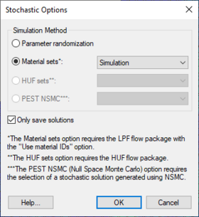
*Select the ''Stochastic Simulation'' from the [[GMS:Global Options/Basic Package|''Global Options'' | *Select the ''Stochastic Simulation'' from the [[GMS:Global Options/Basic Package|''Global Options'' dialog]]. | ||
*Enter the ''Stochastic...'' dialog from the ''MODFLOW'' menu. | *Enter the ''Stochastic...'' dialog from the ''MODFLOW'' menu. | ||


