|
|
| (33 intermediate revisions by 2 users not shown) |
| Line 1: |
Line 1: |
| {{Infobox Calibration}} | | {{Infobox Calibration}} |
| There are two methods in GMS for stochastic modeling using MODFLOW 2000. The first, [[GMS:Stochastic Modeling#Using Parameter Zonation With Stochastic Modeling|parameter zonation]], uses either a [[GMS:Stochastic Modeling#Using Parameter Zonation With Stochastic Modeling|Random Sampling]], [[GMS:Stochastic Modeling#Using Parameter Zonation With Stochastic Modeling|Latin Hypercube Sampling]], or [[GMS:Gaussian Field Generator|Gaussian Fields]] to generate the different realizations. The second approach uses [[GMS:Stochastic Modeling#Using Indicator Simulations With Stochastic Modeling|indicator simulations]] generated by [[GMS:T-PROGS|T-PROGS]]. | | There are three methods in GMS for stochastic modeling using MODFLOW 2000 or 2005. The first, [[GMS:Stochastic Modeling#Using Parameter Zonation With Stochastic Modeling|parameter zonation]], uses either a [[GMS:Stochastic Modeling#Using Parameter Zonation With Stochastic Modeling|random sampling]], a [[GMS:Stochastic Modeling#Using Parameter Zonation With Stochastic Modeling|Latin hypercube sampling]], or [[GMS:Gaussian Field Generator|Gaussian fields]] to generate the different realizations. The second approach uses [[GMS:Stochastic Modeling#Using Indicator Simulations With Stochastic Modeling|indicator simulations]] generated by [[GMS:T-PROGS|T-PROGS]]. The third, the Null Space Monte Carlo (NSMC) method, generates multiple generated models with different sets of parameters (in GMS 9.0 and after). |
|
| |
|
| After the stochastic simulation results are generated, you can view these results using the [[GMS:The GMS Window|Project Explorer]]. You can also refine the results by using the [[GMS:Risk Analysis Wizard|''Risk Analysis Wizard'']] or [[GMS:Stochastic Modeling#Statistical Analysis of Stochastic MODFLOW/MT3D solutions|Statistical Analysis of Stochastic solutions]]. | | After the stochastic simulation results are generated, a user can view these results using the [[GMS:The GMS Window|Project Explorer]]. A user can also refine the results by using the [[GMS:Risk Analysis Wizard|''Risk Analysis Wizard'']] or [[GMS:Stochastic Modeling#Statistical Analysis of Stochastic MODFLOW/MT3D solutions|statistical analysis of stochastic solutions]]. |
| | |
| | The stochastic modeling options can be added to a [http://www.aquaveo.com/software/gms-pricing paid edition] of GMS. |
| | [[Category:Link to Store]] |
|
| |
|
| ==Stochastic Applications== | | ==Stochastic Applications== |
| Line 8: |
Line 11: |
|
| |
|
| The ultimate application of T-PROGS is to generate stochastic simulations of soil heterogeneity. These realizations can then be incorporated into MODFLOW simulations as "material sets" in the [[GMS:LPF Package|LPF package]] or as "HUF data" in the [[GMS:HUF Package|HUF package]]. (See [[GMS:T-PROGS|T-PROGS]]) | | The ultimate application of T-PROGS is to generate stochastic simulations of soil heterogeneity. These realizations can then be incorporated into MODFLOW simulations as "material sets" in the [[GMS:LPF Package|LPF package]] or as "HUF data" in the [[GMS:HUF Package|HUF package]]. (See [[GMS:T-PROGS|T-PROGS]]) |
| | |
| | ==Stochastic Options Dialog== |
| | [[File:GMS StochasticOptions.png|thumb|280 px|The ''Stochastic Options'' dialog]] |
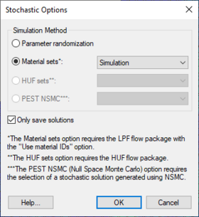
| | Use the ''Stochastic Options'' dialog to select the type of stochastic simulation its major options. The dialog is reached through the ''MODFLOW'' | '''Stochastic''' menu command. |
| | |
| | ''Parameter Randomization'' |
| | : This option uses parameters defined in ''Parameters'' Dialog. |
| | |
| | ''Material Sets'' |
| | : This option becomes available when there is at least one material set simulation in memory. One method for creating material sets is to use [[GMS:T-PROGS|T-PROGS]]. When this stochastic option is chosen, MODFLOW will be run once for each material set. This option also requires that the LPF package and the material IDs option be chosen. |
| | |
| | ''HUF Sets'' |
| | : This option becomes available when there is at least one HUF set simulation in memory. One method for creating HUF sets is to use [[GMS:T-PROGS|T-PROGS]]. When this stochastic option is chosen, MODFLOW will be run once for each HUF set. This option also requires that the HUF package be chosen. |
| | |
| | ''PEST NSMC'' |
| | : In order to use the Null Space Monte Carlo method, there must be a model that has already been calibrated using PEST with SVD-Assist. Selecting this option will cause an '''Options''' button to appear. This button will open the [[GMS:Null Space Monte Carlo|''Monte Carlo Options'']] dialog. |
| | |
| | ''Only Save Solutions'' |
| | : With this option selected, during each stochastic iteration, changes are made to MODFLOW simulation and only a few files are saved. If this option is not selected, each stochastic iteration results in a new entire set of MODFLOW files being saved. |
| | |
| | : Using this option requires less disk space, but doesn't allow loading and rerunning individual stochastic iteration simulations. |
| | |
| | ==Reading Stochastic Solutions== |
| | [[File:GMS - Reading Stochastic Solutions dialog.png|thumb|350 px|The ''Reading Stochastic Solutions'' dialog]] |
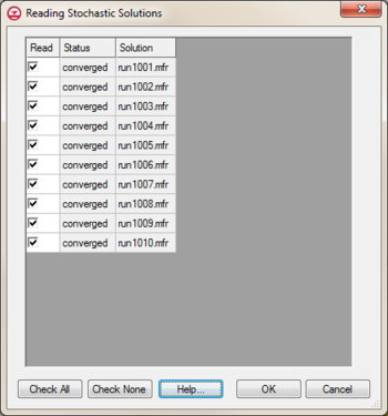
| | At the completion of the model run, if the ''Load Solution'' option is checked, the ''Reading Stochastic Solutions'' dialog will appear when exiting the model wrapper. This dialog gives the option to select which stochastic solutions to load into GMS. Solution not read in at this time can be opened at a later time. |
|
| |
|
| ==Stochastic Inverse Modeling== | | ==Stochastic Inverse Modeling== |
| Line 23: |
Line 51: |
|
| |
|
| The starting heads are interpolated to decrease the run times during the inverse portion. | | The starting heads are interpolated to decrease the run times during the inverse portion. |
|
| |
| ==Stochastic Options Dialog==
| |
| Use the ''Stochastic Options'' dialog to select the type of stochastic simulation its major options.
| |
|
| |
| ===Parameter Randomization===
| |
| This option uses parameters defined in ''Parameters'' Dialog.
| |
|
| |
| ===Material Sets===
| |
| This option becomes available when there is at least one material set simulation in memory. One method for creating material sets is to use [[GMS:T-PROGS|T-PROGS]]. When this stochastic option is chosen, MODFLOW will be run once for each material set. This option also requires that the LPF package and the material IDs option be chosen.
| |
|
| |
| ===HUF Sets===
| |
| This option becomes available when there is at least one HUF set simulation in memory. One method for creating HUF sets is to use [[GMS:T-PROGS|T-PROGS]]. When this stochastic option is chosen, MODFLOW will be run once for each HUF set. This option also requires that the HUF package be chosen.
| |
|
| |
| ===Only Save Solutions===
| |
| With this option selected, during each stochastic iteration, changes are made to MODFLOW simulation and only a few files are saved. If this option is not selected, each stochastic iteration results in a new entire set of MODFLOW files being saved.
| |
|
| |
| Using this option requires less disk space, but doesn't allow loading and rerunning individual stochastic iteration simulations.
| |
|
| |
|
| ==Using Parameter Zonation With Stochastic Modeling== | | ==Using Parameter Zonation With Stochastic Modeling== |
| Line 47: |
Line 58: |
| *[[GMS:Automated Parameter Estimation#4. Define Parameter Zones|Define parameters]] that link with the zones. | | *[[GMS:Automated Parameter Estimation#4. Define Parameter Zones|Define parameters]] that link with the zones. |
| *Select the ''Stochastic Simulation'' option from the [[GMS:Global Options/Basic Package|''Global Options'']] dialog. | | *Select the ''Stochastic Simulation'' option from the [[GMS:Global Options/Basic Package|''Global Options'']] dialog. |
| *Select the Parameter Randomization option from the ''Stochastic Options'' dialog. | | *Select the ''Parameter Randomization'' option from the ''Stochastic Options'' dialog. |
| *Choose whether to use the Random Sampling or Latin Hypercube randomization approaches in the ''Parameters'' dialog. | | *Choose whether to use the ''Random Sampling'' or ''Latin Hypercube'' randomization approaches in the ''Parameters'' dialog. |
| *Save and Run the model. | | *Save and run the model. |
| *View the different model results using the [[GMS:The GMS Window|''Project Explorer'']]. | | *View the different model results using the [[GMS:The GMS Window|Project Explorer]]. |
| *Further analyze the results using the [[GMS:Risk Analysis Wizard|''Risk Analysis Wizard'']]. | | *Further analyze the results using the [[GMS:Risk Analysis Wizard|''Risk Analysis Wizard'']]. |
|
| |
|
| === Random Sampling === | | === Random Sampling === |
|
| |
|
| Random Sampling is the most widely used approach for generating multiple random model simulations. GMS supports both normal and uniform distributions. | | Random sampling is the most widely used approach for generating multiple random model simulations. GMS supports both normal and uniform distributions. |
|
| |
|
| A normal distribution can be defined as: | | A normal distribution can be defined as: |
|
| |
|
| <!--[[Image:normal.GIF]] | | <!--<math>f(x) = \dfrac{1}{\sqrt{2 \pi \sigma}} \text{exp} \left ( - \frac{(x-u)^2}{2 \sigma ^2} \right )</math>--> |
| <math>f(x) = \dfrac{1}{\sqrt{2 \pi \sigma}} \text{exp} \left ( - \frac{(x-u)^2}{2 \sigma ^2} \right )</math>--> | | :[[Image:stochasticeq1.jpg]] |
| [[Image:stochasticeq1.jpg]] | |
|
| |
|
| where σ is the standard deviation, μ is the mean, and x is the value being sampled. A uniform distribution can be defined as: | | where σ is the standard deviation, μ is the mean, and x is the value being sampled. A uniform distribution can be defined as: |
|
| |
|
| <!--[[Image:linear.gif]] | | <!--<math>f(x) = \dfrac{1}{\beta - \alpha}</math>--> |
| <math>f(x) = \dfrac{1}{\beta - \alpha}</math>--> | | :[[Image:stochasticeq2.jpg]] |
| [[Image:stochasticeq2.jpg]] | |
|
| |
|
| where α and β are the bounds of the parameter value x. | | where α and β are the bounds of the parameter value x. |
|
| |
|
| To set up the Random Sampling, specify the mean, standard deviation, and upper and lower bounds for each parameter. Finally, choose how many realizations to generate. | | To set up the random sampling, specify the mean, standard deviation, and upper and lower bounds for each parameter. Finally, choose how many realizations to generate. |
|
| |
|
| === Latin Hypercube === | | === Latin Hypercube === |
|
| |
|
| The Latin Hypercube randomization approach is a method that tries to efficiently probe the probability space for each parameter in a simulation in such a way that there is at least one simulation that represents every probability area for each parameter. | | The Latin hypercube randomization approach is a method that tries to efficiently probe the probability space for each parameter in a simulation in such a way that there is at least one simulation that represents every probability area for each parameter. |
|
| |
|
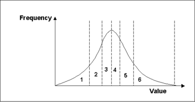
| First, specify the number of segments for each parameter. The total probability, defined by a distribution, mean, standard devation, and upper and lower bounds, is divided up into parts with equal probability (area). GMS then generates a random parameter value so that there is one value that lies within each probability segment. | | First, specify the number of segments for each parameter. The total probability, defined by a distribution, mean, standard devation, and upper and lower bounds, is divided up into parts with equal probability (area). GMS then generates a random parameter value so that there is one value that lies within each probability segment. |
|
| |
|
| [[Image:freq.gif|frame|center|300px]] | | [[Image:freq.png|thumb|none|380px]] |
|
| |
|
| This is repeated in a combinatorial fashion for each parameter so that there are | | This is repeated in a combinatorial fashion for each parameter so that there are |
|
| |
|
| <!--[[Image:combination.gif]] | | <!--<math>\prod_{i=1}^n P_i</math>--> |
| <math>\prod_{i=1}^n P_i</math>--> | | :[[Image:stochasticeq3.jpg]] |
| [[Image:stochasticeq3.jpg]] | |
|
| |
|
| number of simulations, where n is the number of parameters and P is the number of segments for the ith parameter. For example, if there were three parameters with four, four, and five segments, the number of model runs would be as follows: | | number of simulations, where n is the number of parameters and P is the number of segments for the ith parameter. For example, if there were three parameters with four, four, and five segments, the number of model runs would be as follows: |
|
| |
|
| <!--[[Image:comb_example.gif]] | | <!--<math>\ 4*4*5=80</math>--> |
| <math>\ 4*4*5=80</math>--> | | :[[Image:stochasticeq4.jpg]] |
| [[Image:stochasticeq4.jpg]] | |
|
| |
|
| Using the Latin Hypercube method has the benefit of needing a fewer number of runs to achieve the same level of confidence than the number required for the Monte Carlo approach because we have guaranteed that the entire probability range will be explored. | | Using the Latin hypercube method has the benefit of needing a fewer number of runs to achieve the same level of confidence than the number required for the Monte Carlo approach because we have guaranteed that the entire probability range will be explored. |
|
| |
|
| ==Using Indicator Simulations With Stochastic Modeling== | | ==Using Indicator Simulations With Stochastic Modeling== |
| Line 100: |
Line 107: |
| *Generate Material Sets or HUF data using [[GMS:T-PROGS|T-PROGS]]. | | *Generate Material Sets or HUF data using [[GMS:T-PROGS|T-PROGS]]. |
|
| |
|
| *Select the ''Stochastic Simulation'' from the [[GMS:Global Options/Basic Package|''Global Options'' Dialog]]. | | *Select the ''Stochastic Simulation'' from the [[GMS:Global Options/Basic Package|''Global Options'' dialog]]. |
|
| |
|
| *Enter the ''Stochastic...'' dialog from the ''MODFLOW'' menu. | | *Enter the ''Stochastic...'' dialog from the ''MODFLOW'' menu. |
| Line 114: |
Line 121: |
| *GMS will generate as many MODFLOW runs as there are material sets. | | *GMS will generate as many MODFLOW runs as there are material sets. |
|
| |
|
| ==Statistical Analysis of Stochastic MODFLOW/MT3D solutions== | | ==Statistical Analysis of Stochastic MODFLOW/MT3DMS solutions== |
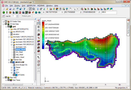
| A statistical analysis can be computed on a Stochastic MODFLOW or MT3D solution by right-clicking on a stochastic folder in the [[GMS:Project Explorer|Project Explorer]] and selecting the '''Statistical Analysis''' command. This command creates four datasets for the mean, min, max, and standard deviation. The 3D grid display options can then be used to visualize these datasets. | | A statistical analysis can be computed on a Stochastic MODFLOW or MT3DMS solution by right-clicking on a stochastic folder in the [[GMS:Project Explorer|Project Explorer]] and selecting the '''Statistical Analysis''' command. This command creates four datasets for the mean, min, max, and standard deviation. The 3D grid display options can then be used to visualize these datasets. |
|
| |
|
| [[Image:StatAnalysis.gif|frame|none|left|500px]] | | [[Image:StatAnalysis.png|thumb|none|left|500px|Stochastic statistical analysis example]] |
|
| |
|
| {{Navbox GMS}} | | {{Navbox GMS}} |
|
| |
|
| [[Category:Stochastic]] | | [[Category:Stochastic|Stochastic GMS]] |
| [[Category:GMS Dialogs|S]] | | [[Category:GMS Stochastic Modeling Dialogs]] |
| [[Category:Equations|S]] | | [[Category:Equations|Stochastic]] |
There are three methods in GMS for stochastic modeling using MODFLOW 2000 or 2005. The first, parameter zonation, uses either a random sampling, a Latin hypercube sampling, or Gaussian fields to generate the different realizations. The second approach uses indicator simulations generated by T-PROGS. The third, the Null Space Monte Carlo (NSMC) method, generates multiple generated models with different sets of parameters (in GMS 9.0 and after).
After the stochastic simulation results are generated, a user can view these results using the Project Explorer. A user can also refine the results by using the Risk Analysis Wizard or statistical analysis of stochastic solutions.
The stochastic modeling options can be added to a paid edition of GMS.
Stochastic Applications
One approach for dealing with model heterogeneity is stochastic simulations based on multiple equally plausible candidate realizations of the site heterogeneity. Ideally, such an approach would enable the generation of variability in subsurface soil stratigraphy based on interpretable geologic parameters such as lens width, material proportions, juxta-positioning tendencies and anisotropy. Multiple realizations that are conditioned to borehole data provide modelers with a rational approach for dealing with uncertainty associated with site characterization. Stochastic simulations can be applied to regional representations of the aquifer behavior in addition to local scale simulations. Stochastic simulations are particularly well-suited to local scale models since the resulting complex heterogeneity is more representative of actual stratigraphic deposition. This heterogeneity makes realistic and potentially more accurate contaminant transport simulation possible by simulating the preferential flow channels resulting from thin lenses of clays, sands, or other materials. The ultimate result of a stochastic approach is multiple simulations of hydraulic parameters that create a probabilistic solution. Such a solution has more credence and provides a better understanding of actual site conditions.
The ultimate application of T-PROGS is to generate stochastic simulations of soil heterogeneity. These realizations can then be incorporated into MODFLOW simulations as "material sets" in the LPF package or as "HUF data" in the HUF package. (See T-PROGS)
Stochastic Options Dialog

The
Stochastic Options dialog
Use the Stochastic Options dialog to select the type of stochastic simulation its major options. The dialog is reached through the MODFLOW | Stochastic menu command.
Parameter Randomization
- This option uses parameters defined in Parameters Dialog.
Material Sets
- This option becomes available when there is at least one material set simulation in memory. One method for creating material sets is to use T-PROGS. When this stochastic option is chosen, MODFLOW will be run once for each material set. This option also requires that the LPF package and the material IDs option be chosen.
HUF Sets
- This option becomes available when there is at least one HUF set simulation in memory. One method for creating HUF sets is to use T-PROGS. When this stochastic option is chosen, MODFLOW will be run once for each HUF set. This option also requires that the HUF package be chosen.
PEST NSMC
- In order to use the Null Space Monte Carlo method, there must be a model that has already been calibrated using PEST with SVD-Assist. Selecting this option will cause an Options button to appear. This button will open the Monte Carlo Options dialog.
Only Save Solutions
- With this option selected, during each stochastic iteration, changes are made to MODFLOW simulation and only a few files are saved. If this option is not selected, each stochastic iteration results in a new entire set of MODFLOW files being saved.
- Using this option requires less disk space, but doesn't allow loading and rerunning individual stochastic iteration simulations.
Reading Stochastic Solutions

The
Reading Stochastic Solutions dialog
At the completion of the model run, if the Load Solution option is checked, the Reading Stochastic Solutions dialog will appear when exiting the model wrapper. This dialog gives the option to select which stochastic solutions to load into GMS. Solution not read in at this time can be opened at a later time.
Stochastic Inverse Modeling
Stochastic inverse modeling is a MODFLOW run option that takes each run in a stochastic simulation and performs parameter estimation on the run to find the optimal values based on observation data. This option is very time consuming compared with a regular stochastic simulation and a parameter estimation run because GMS is doing parameter estimation for each stochastic run times.
Stochastic inverse modeling can be performed only when using material sets or HUF arrays as chosen in the Stochastic Options dialog. PEST is the parameter estimation code supported by GMS.
The following occurs during the stochastic inverse process:
- Run MODFLOW for the stochastic simulation iteration.
- Set the starting head equal to the resulting heads from the MODFLOW run.
- Run parameter estimation.
- Run final MODFLOW (if needed for PEST).
- Move to next stochastic simulation iteration.
The starting heads are interpolated to decrease the run times during the inverse portion.
Using Parameter Zonation With Stochastic Modeling
To create a stochastic MODFLOW simulation using parameter zonation, follow these steps:
- First define the zones using key values.
- Define parameters that link with the zones.
- Select the Stochastic Simulation option from the Global Options dialog.
- Select the Parameter Randomization option from the Stochastic Options dialog.
- Choose whether to use the Random Sampling or Latin Hypercube randomization approaches in the Parameters dialog.
- Save and run the model.
- View the different model results using the Project Explorer.
- Further analyze the results using the Risk Analysis Wizard.
Random Sampling
Random sampling is the most widely used approach for generating multiple random model simulations. GMS supports both normal and uniform distributions.
A normal distribution can be defined as:

where σ is the standard deviation, μ is the mean, and x is the value being sampled. A uniform distribution can be defined as:

where α and β are the bounds of the parameter value x.
To set up the random sampling, specify the mean, standard deviation, and upper and lower bounds for each parameter. Finally, choose how many realizations to generate.
Latin Hypercube
The Latin hypercube randomization approach is a method that tries to efficiently probe the probability space for each parameter in a simulation in such a way that there is at least one simulation that represents every probability area for each parameter.
First, specify the number of segments for each parameter. The total probability, defined by a distribution, mean, standard devation, and upper and lower bounds, is divided up into parts with equal probability (area). GMS then generates a random parameter value so that there is one value that lies within each probability segment.
This is repeated in a combinatorial fashion for each parameter so that there are

number of simulations, where n is the number of parameters and P is the number of segments for the ith parameter. For example, if there were three parameters with four, four, and five segments, the number of model runs would be as follows:

Using the Latin hypercube method has the benefit of needing a fewer number of runs to achieve the same level of confidence than the number required for the Monte Carlo approach because we have guaranteed that the entire probability range will be explored.
Using Indicator Simulations With Stochastic Modeling
GMS allows creating a stochastic simulation using output from T-PROGS. This can be in the form of either material sets or HUF data. Use the following steps:
- Generate Material Sets or HUF data using T-PROGS.
- Enter the Stochastic... dialog from the MODFLOW menu.
- Select the Material Sets option and choose the appropriate material set or HUF data simulation.
- GMS will generate as many MODFLOW runs as there are material sets.
Statistical Analysis of Stochastic MODFLOW/MT3DMS solutions
A statistical analysis can be computed on a Stochastic MODFLOW or MT3DMS solution by right-clicking on a stochastic folder in the Project Explorer and selecting the Statistical Analysis command. This command creates four datasets for the mean, min, max, and standard deviation. The 3D grid display options can then be used to visualize these datasets.

Stochastic statistical analysis example
