GMS:RCH Package: Difference between revisions

From XMS Wiki
Jump to navigationJump to search
No edit summary
No edit summary
 
(9 intermediate revisions by 2 users not shown)
Line 16: Line 16:
; 2D Dataset → Array : The '''2D Dataset → Array''' button brings up the ''Data Browser'' listing all of the current datasets associated with the current 2D grid. In order for this button to be active, the 2D grid must have the same number of rows and columns as the 3D grid. The selected dataset is copied to the recharge array. Datasets are typically generated with the 2D Scatter Point module. The 2D Scatter Point module can be used to interpolate from a scattered set of rainfall measurements to the cell locations. If the dataset is transient, the values in the dataset are linearly interpolated, if necessary, to each stress period as the dataset is copied to the array.


; Array → 2D Dataset : The '''Array → 2D Dataset''' button copies the array to the 2D dataset list associated with the existing 2D grid.
; 3D Dataset → Array : For MODFLOW-USG and MODFLOW-USG Transport only. The '''3D Dataset → Array''' button brings up the ''Select Dataset'' listing all of the current datasets associated with the current 3D grid. In order for this button to be active, the 3D dataset must have the same number of rows and columns as the 3D grid. The selected dataset is copied to the recharge array. Datasets are typically generated with the 3D Scatter Point module. The 3D Scatter Point module can be used to interpolate from a scattered set of rainfall measurements to the cell locations. If the dataset is transient, the values in the dataset are linearly interpolated, if necessary, to each stress period as the dataset is copied to the array.
 
; Array → 2D Dataset : The '''Array → 2D Dataset''' button copies the array to the 2D dataset list associated with the existing 2D grid or UGrid.


; Constant → Array : The '''Constant → Array''' button brings up a dialog which prompts for a single value. This constant is then assigned to each item in the array for the given stress period.
<!-- ; Raster &rarr; Array : The '''Raster &rarr; Array''' button brings up a data browser listing all of the current rasters  
 
-->
; Raster &rarr; Array : The '''Raster &rarr; Array''' button brings up a data browser listing all of the current rasters. Multiple rasters can be selected. After selecting the raster(s) to use, the ''Raster Stress Period Mapping'' dialog will appear. Each raster must be assigned to a stress period. By default, rasters are unassigned.
:If the raster resolution is higher than the grid where there are multiple raster pixels in a grid cell, the pixels will be averaged to get one value for the cell. If it is the other way around, then the grid cell gets the value from the raster pixel that the grid cell center is in. If the raster doesn't cover the whole grid, whatever array values were there before are left unchanged.
 
; Spreadsheet : The recharge flux values for each of the vertical columns in the grid are displayed and edited in the spreadsheet at the lower part of the dialog.


; Reset : The '''Reset''' button deletes all of the data currently defined in the package and restores the package parameters to the default values.
<!--; Reset : The '''Reset''' button deletes all of the data currently defined in the package and restores the package parameters to the default values.-->


Latest revision as of 19:53, 5 March 2024

MODFLOW
Pre-processing
MODFLOW Commands
Building a MODFLOW Model
Map to MODFLOW
Calibration
Packages Supported in GMS
Saving a MODFLOW Simulation
Importing MODFLOW Files
Unsupported MODFLOW Features
Run MODFLOW
Post-processing
MODFLOW Display Options
MODFLOW Post-Processing Viewing Options
Reading a MODFLOW Simulation
Tutorials
Packages
Flow: BCF6, HUF, LPF, UPW
Solvers:

DE4, GMG, NWT, PCG,

PCGN, LMG, SIP, SOR,

SMS
Other:

BAS6, BFH, CHD1, CLN,

DRN1, DRT1, EVT1, ETS1,

GAGE, GHB1, GNC, HFB1,

HUF, LAK3, MNW1, MNW2,

OUT1, RCH1, RIV1, SFR2,

STR1, SUB1, SWI2, WEL1,

UZF1

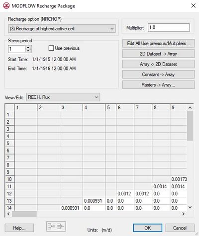
The MODFLOW Recharge Package dialog.

The Recharge package is used to simulate recharge to an aquifer due to rainfall and infiltration. Recharge is typically defined by specifying a recharge value for each stress period for each vertical column in the grid (i.e., a NLAY X NCOL array of values is entered). The recharge value represents the amount of water that goes into the groundwater system and not the amount of precipitation. The units of recharge are length/time, so in a cell with a recharge value of 10(m/day), 10 meters of rainfall each day would be distributed across every m2 of the cell. The recharge parameters are specified in the Recharge Package dialog. The options in the dialog are as follows:

Recharge Option
Three recharge options are supported by MODFLOW: "Recharge only at the top layer", "Recharge at specified vertical cells", and "Recharge at highest active cells".
Multiplier
The multiplier is a constant which can be written to the package file with each stress period array. Each value in the array is scaled by the multiplier as the array is imported to MODFLOW. The format button brings up a dialog listing the standard MODFLOW formats. This format is used for displaying the values in the spreadsheet and it controls how the values are written to the package file.
Stress Periods
The values displayed in the spreadsheet are for an individual stress period. The values associated with other stress periods can be edited by entering the ID of the desired stress period in the Stress period edit box in the center of the dialog. If the Use previous option is selected for a given stress period, the values from the previous stress period are used and the spreadsheet is dimmed.
Layer Indicator
If the Recharge at specified vertical cells option is chosen, the layer indicator for each vertical cell can be displayed and edited in the spreadsheet window by selecting Layer indicator in the View/Edit option.
Edit All Use Previous/Multipliers
This button brings up a spreadsheet allowing the user to edit the Use Previous values and the multipliers for the active array for each stress period.
2D Dataset → Array
The 2D Dataset → Array button brings up the Data Browser listing all of the current datasets associated with the current 2D grid. In order for this button to be active, the 2D grid must have the same number of rows and columns as the 3D grid. The selected dataset is copied to the recharge array. Datasets are typically generated with the 2D Scatter Point module. The 2D Scatter Point module can be used to interpolate from a scattered set of rainfall measurements to the cell locations. If the dataset is transient, the values in the dataset are linearly interpolated, if necessary, to each stress period as the dataset is copied to the array.
3D Dataset → Array
For MODFLOW-USG and MODFLOW-USG Transport only. The 3D Dataset → Array button brings up the Select Dataset listing all of the current datasets associated with the current 3D grid. In order for this button to be active, the 3D dataset must have the same number of rows and columns as the 3D grid. The selected dataset is copied to the recharge array. Datasets are typically generated with the 3D Scatter Point module. The 3D Scatter Point module can be used to interpolate from a scattered set of rainfall measurements to the cell locations. If the dataset is transient, the values in the dataset are linearly interpolated, if necessary, to each stress period as the dataset is copied to the array.
Array → 2D Dataset
The Array → 2D Dataset button copies the array to the 2D dataset list associated with the existing 2D grid or UGrid.
Constant → Array
The Constant → Array button brings up a dialog which prompts for a single value. This constant is then assigned to each item in the array for the given stress period.
Raster → Array
The Raster → Array button brings up a data browser listing all of the current rasters. Multiple rasters can be selected. After selecting the raster(s) to use, the Raster Stress Period Mapping dialog will appear. Each raster must be assigned to a stress period. By default, rasters are unassigned.
If the raster resolution is higher than the grid where there are multiple raster pixels in a grid cell, the pixels will be averaged to get one value for the cell. If it is the other way around, then the grid cell gets the value from the raster pixel that the grid cell center is in. If the raster doesn't cover the whole grid, whatever array values were there before are left unchanged.
Spreadsheet
The recharge flux values for each of the vertical columns in the grid are displayed and edited in the spreadsheet at the lower part of the dialog.