WMS:GSSHA Automated Calibration: Difference between revisions
No edit summary |
No edit summary |
||
| Line 1: | Line 1: | ||
==Auto Calibration== | ==Auto Calibration== | ||
WMS writes the parameters, observed data, and calibration files necessary to run GSSHA in | |||
GSSHA has an automated calibration routine that is described on the GSSHA wiki [http://gsshawiki.com/Alternate_Run_Modes:ERDC_Automated_Model_Calibration_Software here]. WMS writes the parameters, observed data, and calibration files necessary to run GSSHA in any of the supported GSSHA calibration modes. There is a tutorial included in the [[WMS:WMS_Tutorials|WMS Tutorials]] that describes how to setup a basic calibration model. You can enter in the needed data by toggling '''Calibration''' in the ''job control'' dialog. Clicking on the '''Edit Parameters''' button allows you to select which parameters are to be calibrated and edit the calibration settings associated with each of the parameters. The dialog shown below appears, in which you can enter the maximum, minimum, and initial values for each parameter. | |||
[[Image:CalibParams.jpg]] | [[Image:CalibParams.jpg]] | ||
The key for each parameter should be entered in the mapping tables or properties where you desire to calibrate. An example of | The key for each parameter should be entered in the mapping tables or properties where you desire to calibrate. An example of defining keys to calibrate roughness values is shown below. | ||
| Line 17: | Line 18: | ||
Lastly, you | Lastly, you can set the calibration setup parameters, which can be accessed by clicking the '''Calibration Setup...''' button. The following dialog will appear: | ||
| Line 23: | Line 24: | ||
The parameters in this dialog are used for the calibration | The parameters in this dialog are used for the calibration control file. This file, along with the parameters and observed data files are written out by WMS when you save a GSSHA project. | ||
==Manual Calibration== | ==Manual Calibration== | ||
| Line 71: | Line 72: | ||
* [[WMS:GSSHA Observation Points|GSSHA Observation Points]] | * [[WMS:GSSHA Observation Points|GSSHA Observation Points]] | ||
* [[WMS:GSSHA|GSSHA Overview]] | * [[WMS:GSSHA|GSSHA Overview]] | ||
* [[WMS:WMS_Tutorials|WMS Tutorials]] | |||
{{GSSHAMain | {{GSSHAMain | ||
Revision as of 18:48, 26 July 2013
Auto Calibration
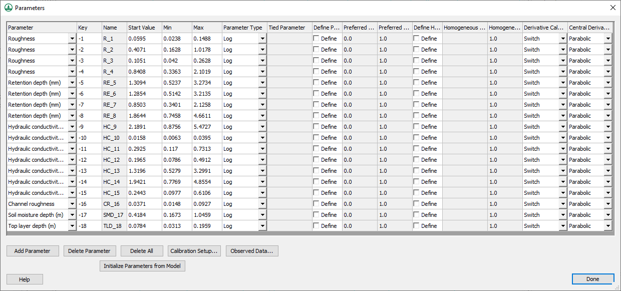
GSSHA has an automated calibration routine that is described on the GSSHA wiki here. WMS writes the parameters, observed data, and calibration files necessary to run GSSHA in any of the supported GSSHA calibration modes. There is a tutorial included in the WMS Tutorials that describes how to setup a basic calibration model. You can enter in the needed data by toggling Calibration in the job control dialog. Clicking on the Edit Parameters button allows you to select which parameters are to be calibrated and edit the calibration settings associated with each of the parameters. The dialog shown below appears, in which you can enter the maximum, minimum, and initial values for each parameter.
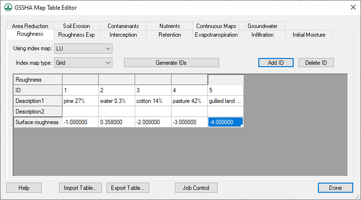
The key for each parameter should be entered in the mapping tables or properties where you desire to calibrate. An example of defining keys to calibrate roughness values is shown below.
Clicking the Observed Data... button in the calibration parameters dialog opens another dialog, which is shown below. In this dialog you can enter in various types of observed data for each event of the simulation.
Lastly, you can set the calibration setup parameters, which can be accessed by clicking the Calibration Setup... button. The following dialog will appear:
The parameters in this dialog are used for the calibration control file. This file, along with the parameters and observed data files are written out by WMS when you save a GSSHA project.
Manual Calibration
Manual calibration is the process of changing simulation input so that the simulation output matches observed values. Manual calibration takes a lot of experience and a lot of patience, but it is possible to achieve a good fit between the simulation and the observed data. Being able to successfully manually calibrate a simulation is a necessary skill to successfully set up and run an automatic calibration program.
Steps in the Manual Calibration Process
- Set up and run a successful simulation.
- Identify the calibration variables.
- Decide on a valid range for each variable.
- Set initial values of variables and run the model.
- Compare model results to observed values.
- Change variable values and re-run.
- Repeat steps 5 and 6 until the simulation results closely approximate the observed values.
1. Set up and run a successful simulation
The first step to calibrating a simulation is to set up and successfully run a reasonable simulation. All known parameters, such as precipitation, should be defined; all unknown parameters should be set to physically realistic values. For example, if actual roughness values are unknown then set all of the roughness values to 0.035 or some other reasonable number. Setting the roughness values to 0.00 or some default value will not allow the simulation to proceed. One important consideration is that if the spatial or temporal resolution is too coarse than the simulation will be unduly influenced by numerical issues related to the implementation of the partial differential equations. The result of too coarse of a temporal or spatial resolution will be delayed flows. For more information, see the Primer: Using Watershed Modeling System (WMS) for Gridded Surface Subsurface Hydrologic Analysis (GSSHA) Data Development – WMS 6.1 and GSSHA 1.43c (Downer et. al 2003).
2. Identify the calibration variables
The calibration variables are the simulation parameters whose exact quantities are unknown. This may range from a small handful to several dozen. At this stage it is also often necessary to identify which parameters the simulation is sensitive to and which can be left at good approximations without unduly affecting the model. The number of calibration variables must be pared down to a manageable number as well. Attempting to manually calibrate a simulation with dozens of unknown parameters will lead to one major headache and not to a good, robust simulation. Calibration cannot overcome a general lack of data.
Occasionally lab tests for such parameters as hydraulic conductivity will be available. Such data is very valuable but it still may be necessary to calibrate on that specific parameter because a simulation parameter represents a uniform parameter over an area while lab results generate the parameter for a specific point. The lab data is a very good starting value but may need some modification before it is applicable to a general area.
3. Decide on a valid range for each variable
Knowing a range for each variable is very important. To accurately simulate what is actually present in the watershed requires knowledge of the physical meaning of all of the numerical parameters for the watershed. Without this understanding a simulation that does not accurately reflect reality will be created and the simulation will be worthless in a predictive capacity. Consulting published works that describe the formulas used in GSSHA and detail the values and physical meaning of the formula parameters is highly recommended.
4. Set initial values of variables and run the model
Once the calibration variables have been decided upon and the valid range for each has been identified, the next step is to set an initial value for each variable. The usual process is to begin with the middle value. Later on these values will be modified little by little, either up or down. Beginning with the middle value of the range gives a good reference point for later simulations where what happens with a higher or lower value can be judged against the middle value to determine simulation trends.
5. Compare model results to observed values
This is the key step to calibrating a simulation. Click on the button in the Solution Results column of the Feature Point/Node Properties dialog to display the Solution Analysis dialog, which allows both visual inspection of the solution result as well as numerical evaluation of the “fitness” of a solution. Using these criteria judge how well the simulation output fits the observed.
6. Change variables and re-run
If the simulation output is not sufficiently close to the observed data then the next step is to adjust one or more of the model parameters to try to get a better fit. This step takes practice, experience, and patience. If by adjusting the variables outside of the predefined range a better fit is obtained then either the simulation is poorly set up or the data on which the model is based may be in question. It may also be that the interdependence of variables is such that the other variables in the model should be adjusted before the one that seems to call into question the parameter bounds. After adjusting the variables and running the simulation, check the new output and judge the results of the new variable setting.
Simulation non-uniqueness
One important facet of calibrating a simulation is that often changing more than one variable can have very similar results on the simulation output. Calibrating a simulation attempts to extract spatial simulation parameters from observed data through a process called inverse modeling. Problems arise in calibrating when modifying more than one variable produces only one type of result in the simulation. The question then arises as to which variable values should be the actual variable values. This problem is not solvable and the simulation is said to be non-unique or over-specified. The only way to overcome this problem is by utilizing more data that is of a different type than that already being used. For example, using a stream-flow hydrograph as well as a set of observed groundwater elevations would help eliminate simulation non-uniqueness.
Related Topic
GSSHA | |
|---|---|
| XMS Wiki Links | Calibration (Automated • Manual • Output) • Channel Routing • Contaminants • Digital Dams • Embankment Arcs • Feature Objects (Arcs • Nodes • Polygons) • File Types • Groundwater • Groups • Hydraulic Structures • Job Control • Join SSURGO Data • Mapping Tables • Maps • Menu • Model Linkage • Multiple Simulations • Nutrients • Observations • Output Control • Overland Soil Erosion • Pipe and Node Parameters • Precipitation • Radar Rainfall • Save GSSHA Project File • Smooth GSSHA Streams • Snowmelt • Solution (Analysis • Data) |
| Related Tools | MWBM Wizard • Using Soil Type Data with GSSHA |
| GSSHA Wiki External Links | GSSHA Wiki: Overview • Primer • User's Manual • Tutorials |


