WMS:GSSHA: Difference between revisions
No edit summary |
|||
| Line 28: | Line 28: | ||
Note: GSSHA currently supports file names (including path and file name) with lengths less than or equal to 128 characters. If GSSHA tutorial files are placed in a directory with a path that causes the combined path and file name to exceed 128 characters, then GSSHA will not run. | Note: GSSHA currently supports file names (including path and file name) with lengths less than or equal to 128 characters. If GSSHA tutorial files are placed in a directory with a path that causes the combined path and file name to exceed 128 characters, then GSSHA will not run. | ||
==Save Project File== | ===Save Project File=== | ||
Specify the GSSHA project file name and location in the ''Save GSSHA Project File'' dialog. Select ''Save'' to save the GSSHA project file and all other GSSHA input files. WMS automatically uses the GSSHA project file name as a prefix for all GSSHA input files (file extensions are used to differentiate between GSSHA input files), except for the index map files, which are assigned default names using the convention id_map_##.idx, where ## is generated by WMS. All files are written to the same directory according to the specified location. | Specify the GSSHA project file name and location in the ''Save GSSHA Project File'' dialog. Select ''Save'' to save the GSSHA project file and all other GSSHA input files. WMS automatically uses the GSSHA project file name as a prefix for all GSSHA input files (file extensions are used to differentiate between GSSHA input files), except for the index map files, which are assigned default names using the convention id_map_##.idx, where ## is generated by WMS. All files are written to the same directory according to the specified location. | ||
Revision as of 20:46, 15 March 2019
GSSHA is a two-dimensional finite difference rainfall/runoff model. A finite difference grid is used to establish the computational domain and parameters for surface runoff. The GSSHA model is fully coupled with hydraulic stream flow/routing models. Parameters for stream channels are defined using arcs and then mapped to the appropriate underlying grid cells.
According to the GSSHA wiki overview page, "features include two dimensional (2-D) overland flow, 1-D stream flow, 1-D infiltration, 2-D groundwater, and full coupling between the groundwater, shallow soils, streams, and overland flow. Sediment and constituent fate and transport are simulated in the shallow soils, overland flow plane, and in streams and channels. GSSHA can be used as an episodic or continuous model where soil surface moisture, groundwater levels, stream interactions, and constituent fate are continuously simulated. The fully coupled groundwater to surface-water interaction allows GSSHA to model basins in both arid and humid environments."[1]
A detailed online reference manual for GSSHA is found here: http://www.gsshawiki.com
The GSSHA model can be added to a paid edition of WMS.
GSSHA Menu
Open Project File
The Open Project File command in the GSSHA menu looks for a GSSHA project file. A GSSHA project file begins with the first line either being GSSHAPROJECT or CASC2DPROJECT. Once a valid project file has been identified, WMS will read in all of the files needed for input to GSSHA. The channel input file is not read in but instead the channel input information is re-created from the WMS map file that stores the GSSHA coverage. GSSHA output files are not read in by the Open Project File command but instead are read by the Read Solution command.
Model Check
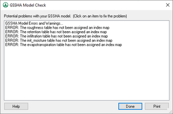
The GSSHA | Model Check command runs through the input data for a GSSHA simulation and looks for obvious inconsistencies and problems with the model. The model checker will not identify values that are outside of plausible ranges, etc., only logical problems. For example, an index map has one or more cells whose ID is 0 (which is not allowed in GSSHA), or a specified process that has an ID with parameters whose values are 0.00 (which indicates an incomplete entry). An example of a problem that the model checker would not find is if a stream arc has a pit that pools water.
Run Simulation
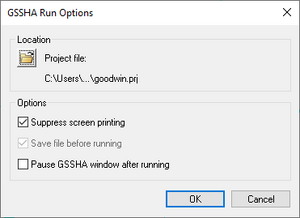
The Run GSSHA command launches GSSHA in the WMS model wrapper. Select an existing GSSHA project file or specify the name and location of the GSSHA project file to be saved before running the simulation. The GSSHA Run Options include:
- Suppress screen printing
- Save files before running
- Pause GSSHA window after running
The Suppress screen printing option suppresses the output of runtime data from GSSHA at each time step, but significantly reduces the overall run time required for a GSSHA simulation. This option also requires that the GSSHA input files be saved before running the simulation.
WMS will automatically read the GSSHA solution produced by the simulation when the Close button is clicked in the WMS Model Wrapper if the Read Solution on Exit option is toggled on.
Note: GSSHA currently supports file names (including path and file name) with lengths less than or equal to 128 characters. If GSSHA tutorial files are placed in a directory with a path that causes the combined path and file name to exceed 128 characters, then GSSHA will not run.
Save Project File
Specify the GSSHA project file name and location in the Save GSSHA Project File dialog. Select Save to save the GSSHA project file and all other GSSHA input files. WMS automatically uses the GSSHA project file name as a prefix for all GSSHA input files (file extensions are used to differentiate between GSSHA input files), except for the index map files, which are assigned default names using the convention id_map_##.idx, where ## is generated by WMS. All files are written to the same directory according to the specified location.
For long term simulations WMS copies the HMET file from its original location to the new GSSHA project directory.
It is also possible to manage all of the GSSHA input and output files names using the Manage files option in the GSSHA Job Control Parameters dialog.
GSSHA Files
Here are tables of some of the available files for GSSHA.
- For more information on these files see the GSSHA online manual
| Name | Description |
|---|---|
| PRJ | GSSHA Project File |
| TRE | WMS Tree File |
| STO | WMS Stochastic Information File |
| MAP | WMS Map File |
| OUT | GSSHA Output Summary File |
| IDX | GSSHA Cell Index File |
| PRO | GSSHA Projectioin File |
| OTL | GSSHA Outlet Series Discharge File |
| MSK | GSSHA Watershed Delineation Mask File |
| ELE | GSSHA Cell Elevation File |
| DEP | GSSHA Depth File |
| CMT | GSSHA Area Property Mapping Table File |
Read Solution
While solutions are not new to GSSHA, being able to work with them in WMS is a new feature. Accessible from the GSSHA menu in the 2D grid module is the command Read Solution which looks for a GSSHA project file and then reads in all of the associated datasets and lumps them together into a solution folder in the Project Explorer. Solution folders are identified by a lowercase "s" on the folder. All of the datasets in the folder are treated as regular datasets. Organizing the datasets into a solution allows several solutions to be in memory at the same time. Several dialogs look for solutions and the associated datasets to set up and display output graphs. Along with the regular datasets, the summary file for the project is also accessible for each solution by double-clicking the summary file project explorer item under the solution folder.
Individual solution output time series data for a cell may be viewed from the Solution Results dialog accessed from the Feature Point/Node Type dialog. This dialog will only show the output dataset time series for the cell that underlies the feature point selected. To compare the solution output at a cell with observed data, see the GSSHA Observation Points section.
Cell Properties
The 2D grid cell properties include an I, J location and a scalar or index map value. The scalar or index map value is associated with the currently selected dataset in the Project Explorer and can be edited in the Properties Window. The I, J location can be viewed but cannot be edited in the Properties Window. The 2D grid contours are a way of visualizing the spatial variation of the scalar or index map values for the selected dataset.
Related Topics
- GSSHA Calibration
- GSSHA Channel Routing
- GSSHA Contaminants
- GSSHA Digital Dams
- GSSHA Embankment Arcs
- GSSHA Groundwater
- GSSHA Maps
- GSSHA Job Control
- GSSHA Model Linkage
- GSSHA Join SSURGO Data
- GSSHA Mapping Tables
- GSSHA Maps
- GSSHA Multiple Scenarios
- GSSHA Nutrients
- GSSHA Overland Soil Erosion
- GSSHA Output Control
- GSSHA Precipitation
- GSSHA Solution Analysis
GSSHA | |
|---|---|
| XMS Wiki Links | Calibration (Automated • Manual • Output) • Channel Routing • Contaminants • Digital Dams • Embankment Arcs • Feature Objects (Arcs • Nodes • Polygons) • File Types • Groundwater • Groups • Hydraulic Structures • Job Control • Join SSURGO Data • Mapping Tables • Maps • Menu • Model Linkage • Multiple Simulations • Nutrients • Observations • Output Control • Overland Soil Erosion • Pipe and Node Parameters • Precipitation • Radar Rainfall • Save GSSHA Project File • Smooth GSSHA Streams • Snowmelt • Solution (Analysis • Data) |
| Related Tools | MWBM Wizard • Using Soil Type Data with GSSHA |
| GSSHA Wiki External Links | GSSHA Wiki: Overview • Primer • User's Manual • Tutorials |

