User:Jmonson/MODFLOW 6 Packages: Difference between revisions
No edit summary |
(→UZF) |
||
| Line 319: | Line 319: | ||
{{-}} | {{-}} | ||
===UZF=== | ===UZF=== | ||
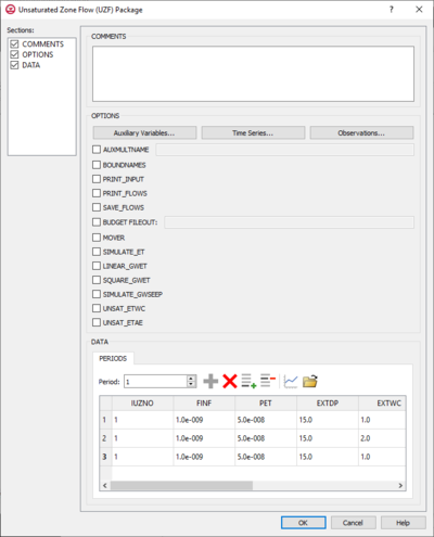
[[File: | [[File:MF6-UZF package.png|thumb|400px|right|The ''Unsaturated Zone Flow (UZF)'' dialog]] | ||
{{-}} | {{-}} | ||
===WEL=== | ===WEL=== | ||
[[File:MF6-WellsPackageDialog.png|thumb|400px|right|The ''Well (WEL) Package'' dialog]] | [[File:MF6-WellsPackageDialog.png|thumb|400px|right|The ''Well (WEL) Package'' dialog]] | ||
Revision as of 21:59, 5 February 2020
| This contains information about future features. |
| MODFLOW | |
|---|---|
| Pre-processing | |
| MODFLOW Commands | |
| Building a MODFLOW Model | |
| Map to MODFLOW | |
| Calibration | |
| Packages Supported in GMS | |
| Saving a MODFLOW Simulation | |
| Importing MODFLOW Files | |
| Unsupported MODFLOW Features | |
| Run MODFLOW | |
| Post-processing | |
| MODFLOW Display Options | |
| MODFLOW Post-Processing Viewing Options | |
| Reading a MODFLOW Simulation | |
| Tutorials | |
| Packages | |
| Flow: | BCF6, HUF, LPF, UPW |
| Solvers: | SMS |
| Other: | UZF1 |
There are many different packages available in MODFLOW 6.
Contents
- 1 Packages
- 1.1 Temporal Discretization (TDIS) Package
- 1.2 Iterative Model Solution (IMS)
- 1.3 Structured Discretization (DIS) Package
- 1.4 Node Property Flow (NPF) Package
- 1.5 Initial Conditions (IC) Package
- 1.6 Constant-Head (CHD) Package
- 1.7 Drain (DRN) Package
- 1.8 EVT
- 1.9 GHB
- 1.10 GNC
- 1.11 HFB
- 1.12 LAK
- 1.13 MAW
- 1.14 MVR
- 1.15 OBS
- 1.16 OC
- 1.17 RCH
- 1.18 RIV
- 1.19 SFR
- 1.20 STO
- 1.21 UZF
- 1.22 WEL
- 1.23 ZONE FILE
- 2 Date/Time Dialog
- 3 Auxiliary Variables Dialog
- 4 Time Series Files Dialog
- 5 Observation Files Dialog
- 6 Add Stresses Dialog
- 7 External Link
Packages
Temporal Discretization (TDIS) Package
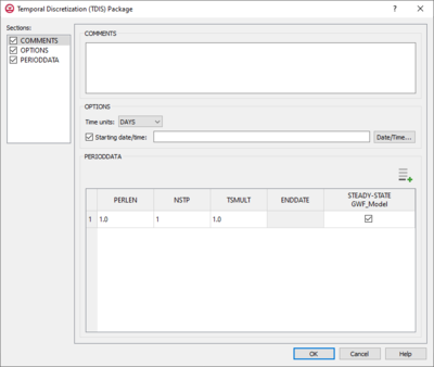
The Temporal Discretization (TDIS) Package dialog is accessed by double-clicking on the TDIS package under a MODFLOW 6 simulation in the Project Explorer. It contains the following sections and options:
- Sections list – A list of sections that can be turned on or off:
- Comments – Turn on to make the Comments section visible.
- Options – Turn on to make the Options section visible.
- PeriodData – Turn on to make the PeriodData section visible. This section is on by default.
- Comments section – Enter general alphanumeric comments. Comments entered here get written at the top of the file, preceded by a '#' symbol.
- Options section – Temporal options and settings:
- Time units drop-down – A drop-down menu with the following options for the type of time units:
- "Unknown"
- "Seconds"
- "Minutes"
- "Hours"
- "Days" – The default selection.
- "Years"
- Start date/time – Turn on to enable setting a start date/time. Click the Date/Time... button to bring up the Date/Time dialog. The time can also be manually entered using "YYYY-MM-DDTHH:MM:SS" format. The "T" in the middle divides the date from the time.
- Time units drop-down – A drop-down menu with the following options for the type of time units:
- PeriodData section – Contains a spreadsheet listing periods. An
 Add Row button is found at the top rigth of the spreadsheet. Right-clicking on the row number in the spreadsheet gives a menu that allows inserting, deleting, copying, or pasting a row. The columns in the spreadsheet include:
- PERLEN – The length of a stress period. The default value is "1.0".
- NSTP – The number of time steps in a stress period. The default value is "1".
- TSMULT – The multiplier for the length of successive time steps. The default value is "1.0".
- ENDDATE – The end date for that period. This field is not directly user-editable, but will automatically change if the PERLEN value is changed.
- STEADY-STATE GWF_Model – Turn on if the period is steady state and using the GWF Model.
Iterative Model Solution (IMS)
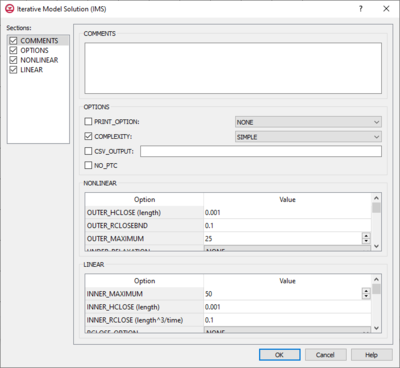
The Iterative Model Solution (IMS) dialog is accessed by double-clicking on the IMS package under a MODFLOW 6 simulation in the Project Explorer. It contains the following sections and options:
- Sections list – A list of sections that can be turned on or off:
- Comments – Turn on to make the Comments section visible.
- Options – Turn on to make the Options section visible.
- Nonlinear – Turn on to make the Nonlinear section visible. This section is on by default.
- Linear – Turn on to make the Linear section visible. This section is on by default.
- Comments section – Enter general alphanumeric comments. Comments entered here get written at the top of the file, preceded by a '#' symbol.
- Options section
- PRINT_OPTION – A flag that controls printing of convergence information from the solver. Turn on to make the following print options available from the drop-down:
- "None" – Print nothing. This is the default when PRINT_OPTION is not turned on.
- "Summary" – Print only the total number of iterations and nonlinear residual reduction summaries
- "All" – Print linear matrix solver convergence information to the solution listing file and model specific linear matrix solver convergence information to each model listing file in addition to "Summary" information.
- COMPLEXITY – Optional. Defines default non-linear and linear solver parameters. Turn on to make the following options available from the drop-down:
- "Simple" – Default solver input values will be defined that work well for nearly linear models.
- "Moderate" – Default solver input values will be defined that work well for moderately nonlinear models.
- "Complex" – Default solver input values will be defined that work well for highly nonlinear models.
- CSV_OUTPUT – Turn on to specify that the record corresponds to the comma separated values solver convergence output. Enter the desired filename for the output ASCII CSV file in the empty field to the right of the option.
- NO_PTC – Turn on to disable pseudo-transient continuation (PTC). Only applies to steady-state stress periods for models using the Newton-Raphson formulation.
- PRINT_OPTION – A flag that controls printing of convergence information from the solver. Turn on to make the following print options available from the drop-down:
- Nonlinear section – A table with two columns: "Option" (giving the name of the option) and "Value", where a value can be entered for the option. The options include the following:
- OUTER_HCLOSE (length) – Real value defining the head change criterion for convergence of the outer (nonlinear) iterations, in units of length. Default value is "0.001".
- OUTER_RCLOSEBND – Real value defining the residual tolerance for convergence of model packages that solve a separate equation not solved by the IMS linear solver. Default value is "0.1"
- OUTER_MAXIMUM – Integer value defining the maximum number of outer (nonlinear) iterations. Default value is "25".
- UNDER_RELAXATION – Optional drop-down value. Defines the nonlinear under-relaxation schemes used.
- "None" – Under-relaxation is not used.
- "Simple" – Simple under-relaxation scheme with a fixed relaxation factor is used.
- "Cooley" – Cooley under-relaxation scheme is used.
- "DBD" – Delta-bar-delta under-relaxation is used.
- UNDER_RELAXATION_THETA – Real value defining the reduction factor for the learning rate (under-relaxation term) of the delta-bar-delta algorithm. Default value is "0.0".
- UNDER_RELAXATION_KAPPA – Real value defining the increment for the learning rate (under-relaxationterm) of the delta-bar-delta algorithm. Default value is "0.0".
- UNDER_RELAXATION_GAMMA – Real value defining the history or memory term factor of the delta-bar-delta algorithm. Default value is "0.0".
- UNDER_RELAXATION_MOMENTUM – Real value defining the fraction of past history changes that is added as a momentum term to the step change for a nonlinear iteration. Default value is "0.0".
- BACKTRACKING_NUMBER – Integer value defining the maximum number of backtracking iterations allowed for residual reduction computations. Default value is "0".
- BACKTRACKING_TOLERANCE – Only available if BACKTRACKING_NUMBER" has a value of "1" or higher. Real value defining the tolerance for residual change that is allowed for residual reduction computations
- BACKTRACKING_REDUCTION_FACTOR – Only available if BACKTRACKING_NUMBER" has a value of "1" or higher. Real value defining the reduction in step size used for residual reduction computations
- BACKTRACKING_RESIDUAL_LIMIT – Only available if BACKTRACKING_NUMBER" has a value of "1" or higher. Real value defining the limit to which the residual is reduced with backtracking.
- Linear section – A table with two columns: "Option" (giving the name of the option) and "Value", where a value can be entered for the option. The options include the following:
- INNER_MAXIMUM – Integer value defining the maximum number of inner (linear) iterations. Default value of "50".
- INNER_HCLOSE (length) – Real value defining the head change criterion for convergence of the inner (linear) iterations, in units of length. Default value of "0.001".
- INNER_RCLOSE (length3/time) – Real value that defines the flow residual tolerance for convergence of the IMS linear solver and specific flow residual criteria used. Default value of "0.1".
- RCLOSE_OPTION – Optional. Defines the specific flow residual criterion used. Default selection of "None". Has the following options:
- "None" – If selected, an absolute residual (infinity-norm) criterion is used.
- "Strict" – Specifies that INNERRCLOSE represents an infinity-Norm (absolute convergence criteria) and that the head and flow convergence criteria must be met on the first inner iteration.
- "L2NORM_RCLOSE" – Specifies that INNERRCLOSE represents a L-2 Norm closure criteria instead of an infinity-Norm (absolute con-vergence criteria).
- "RELATIVE_RCLOSE" – Spcifies that INNERRCLOSE represents a relative L-2 Norm reduction closure criteria instead of an infinity-Norm (absolute convergence criteria).
- LINEAR_ACCELERATION – Defines the linear acceleration method used by the default IMS linear solvers. Default selection of "CG". Has the following options:
- "CG" – Preconditioned conjugate gradient method.
- "BICGSTAB" – Preconditionedbi-conjugate gradient stabilized method.
- RELAXATION_FACTOR – Optional. Real value that defines the relaxation factor used by the incomplete LU factorization preconditioners (MILU(0) and MILUT). Default value of "0.0".
- PRECONDITIONER_LEVELS – Optional. Integer value defining the level of fill for ILU decomposition used in the ILUT and MILUT preconditioners. Default value of "0".
- PRECONDITIONER_DROP_TOLERANCE – Optional. Real value that defines the drop tolerance used to drop preconditioner terms based on the magnitude of matrix entries in the ILUT and MILUT preconditioners. Default value of "0.0".
- NUMBER_ORTHOGONALIZATIONS – Optional. Integer value defining the interval used to explicitly recalculate the residual of the flow equation using the solver coefficient matrix, the latest head estimates, and the right hand side. Default value of "0".
- SCALING_METHOD – Optional. Defines the matrix scaling approach used. Default selection of "None". Has the following options:
- "None" – No matrix scaling applied.
- "Diagonal" – Symmetric matrix scaling using the POLCG preconditioner scaling method.
- "L2NORM" – Symmetric matrix scaling using the L2 norm.
- REORDERING_METHOD – Optional. Defines the matrix reordering approach used. Default selection of "None". Has the following options:
- "None" – Original ordering.
- "RCM" – Reverse Cuthill McKee ordering.
- "MD" – Minimum degree ordering.
Structured Discretization (DIS) Package
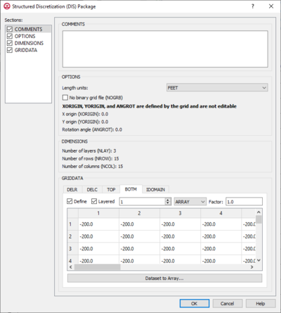
The Structured Discretization (DIS) Package dialog is accessed by double-clicking on the DIS package under a MODFLOW 6 simulation in the Project Explorer. It contains the following sections and options:
- Sections list – A list of sections that can be turned on or off:
- Comments – Turn on to make the Comments section visible.
- Options – Turn on to make the Options section visible.
- Dimensions – Turn on to make the Dimensions section visible.
- GridData – Turn on to make the GridData section visible. This section is on by default.
- Comments section – Enter general alphanumeric comments. Comments entered here get written at the top of the file, preceded by a '#' symbol.
- Options' section
- Length units – A drop-down with options specifying the length units used for this model:
- "Feet"
- "Meters"
- "Centimeters"
- "Unknown"
- No binary grid file (NOGRB) – Turn on to deactivate writing of the binary grid file.
- X origin (XORIGIN) – Defined by the grid and not user editable here.
- Y origin (YORIGIN) – Defined by the grid and not user editable here.
- Rotation angle (ANGROT) – Defined by the grid and not user editable here.
- Length units – A drop-down with options specifying the length units used for this model:
- Dimensions section – This is an informational section displaying the number of layers (NLAY), number of rows (NROW), and number of columns (NCOL). These are defined by the grid and not user editable here.
- GridData section – Contains a number of tabs, including:
- DELR – Column spacing in the row direction. Defined by the grid and not user editable here.
- DELC – Row spacing in the column direction. Defined by the grid and not user editable here.
- TOP – Top elevation for each cell in the top model layer.
- Layered – This option is not available as there is only one top layer.
- If "Constant" is selected from the drop-down, enter a decimal value in the Constant field to be applied to all cells in the top model layer.
- If "Array" is selected from the drop-down, a user-editable array appears below the drop-down. Enter a decimal Factor value to the right of the drop-down. The individual elements of the array are multiplied by the factor value after they are read.
- BOTM – Bottom elevation for each cell.
- Layered – Turn on if there is more than one bottom layer. Select the desired layer from the drop down in order to edit the array (if "Array" is selected from the drop-down).
- If "Constant" is selected from the drop-down, enter a decimal value in the Constant field to be applied to all cells in the bottom model layer(s).
- If "Array" is selected from the drop-down, a user-editable array appears below the drop-down. Enter a decimal Factor value to the right of the drop-down. The individual elements of the array are multiplied by the factor value after they are read.
- Dataset to Array... – Click to open the Select Dataset dialog. Select the desired database(s) and click OK to close the Select Dataset dialog.
- IDOMAIN – Optional. Characterizes the existence status of a cell. Setting a value of "0" for a particular cell inactivates that cell so it is not used in the simulation.
- Define – Turn on to define an IDOMAIN.
- Layered – Turn on if there is more than one bottom layer. Select the desired layer from the drop down in order to edit the array (if "Array" is selected from the drop-down).
- If "Constant" is selected from the drop-down, enter a decimal value in the Constant field to be applied to all cells in the IDOMAIN layer(s).
- If "Array" is selected from the drop-down, a user-editable array appears below the drop-down. Enter a decimal Factor value to the right of the drop-down. The individual elements of the array are multiplied by the factor value after they are read.
- Dataset to Array... – Click to open the Select Dataset dialog. Select the desired database(s) and click OK to close the Select Dataset dialog.
Node Property Flow (NPF) Package
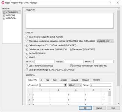
The Node Property Flow (NPF) Package dialog is accessed by double-clicking on the NPF package under a MODFLOW 6 simulation in the Project Explorer. It contains the following sections and options:
- Sections list – A list of sections that can be turned on or off:
- Comments – Turn on to make the Comments section visible.
- Options – Turn on to make the Options section visible.
- GridData – Turn on to make the GridData section visible. This section is on by default.
- Comments section – Enter general alphanumeric comments. Comments entered here get written at the top of the file, preceded by a '#' symbol.
- Options section
- Save flows to budget file (SAVE_FLOWS) – Turn on to write cell-by-cell flow terms to the file specified with "BUDGET SAVE FILE" in Output Control.
- Alternative conductance calculation method (ALTERNATIVE_CELL_AVERAGING) – Turn on to use an alternative method for calculating the conductance for horizontal cell connections.
- "Logarithmic" –
- "AMT-LMK" – Conductance will be calculated using arithmetic-mean thickness and logarithmic-mean hydraulic conductivity.
- "AMT-HMK" – Conductance will be calculated using arithmetic-mean thickness and harmonic-mean hydraulic conductivity.
- Cells with negative ICELLTYPE are confined (THICKSTRT) – Cells having a negative ICELLTYPE are confined, and their cell thickness for conductance calculations will be computed as STRT-BOT rather than TOP-BOT.
- Calculate vertical conductance (VARIABLECV) – Vertical conductance will be calculated using the saturated thickness and properties of the overlying cell and the thickness and properties of the underlying cell.
- Dewatered (DEWATERED) – Vertical conductance is calculated using only the saturated thickness and properties of the overlying cell if the head in the underlying cell is below its top.
- Perched (PERCHED) – When a cell is overlying a dewatered convertible cell, the head difference used in Darcy's Law is equal to the head in the overlying cell minus the bottom elevation of the overlying cell.
- REWET – Turn on to activate model rewetting.
- WETFCT – A factor included in the calculation of the head, initially established at a cell when that cell is converted from dry to wet.
- IWETIT – Iteration interval for attempting to wet cells.
- IHDWET – Integer flag that determines which equation is used to define the initial head at cells that become wet.
- Use XT3D formulation (XT3D) – Turn on to use the XT3D formulation.
- Add XT3D terms to right-hand side (RHS) – The XT3D additional terms will be added to the right-hand side instead of the coefficient matrix.
- Save specific discharge (SAVE_SPECIFIC_DISCHARGE) – Turn on to calculate x, y, and z components of specific discharge at cell centers and write them to the cell-by-cell flow file as specified with "BUDGET SAVE FILE" in Output Control.
- GridData section – Contains a number of tabs, including:
- ICELLTYPE – A flag for each cell that specifies how saturated thickness is treated.
- Layered – Turn on if there is more than one affected layer. Select the desired layer from the drop down in order to edit the array (if "Array" is selected from the drop-down).
- If "Constant" is selected from the drop-down, enter a decimal value in the Constant field to be applied to all cells in the layer(s).
- If "Array" is selected from the drop-down, a user-editable array appears below the drop-down. Enter a decimal Factor value to the right of the drop-down. The individual elements of the array are multiplied by the factor value after they are read.
- Dataset to Array... – Click to open the Select Dataset dialog. Select the desired database(s) and click OK to close the Select Dataset dialog.
- K – The hydraulic conductivity.
- Layered – Turn on if there is more than one affected layer. Select the desired layer from the drop down in order to edit the array (if "Array" is selected from the drop-down).
- If "Constant" is selected from the drop-down, enter a decimal value in the Constant field to be applied to all cells in the layer(s).
- If "Array" is selected from the drop-down, a user-editable array appears below the drop-down. Enter a decimal Factor value to the right of the drop-down. The individual elements of the array are multiplied by the factor value after they are read.
- Dataset to Array... – Click to open the Select Dataset dialog. Select the desired database(s) and click OK to close the Select Dataset dialog.
- K22 – The hydraulic conductivity of the second ellipsoid axis.
- Define – Turn on if K22 needs to be defined.
- Layered – Turn on if there is more than one affected layer. Select the desired layer from the drop down in order to edit the array (if "Array" is selected from the drop-down).
- If "Constant" is selected from the drop-down, enter a decimal value in the Constant field to be applied to all cells in the layer(s).
- If "Array" is selected from the drop-down, a user-editable array appears below the drop-down. Enter a decimal Factor value to the right of the drop-down. The individual elements of the array are multiplied by the factor value after they are read.
- Dataset to Array... – Click to open the Select Dataset dialog. Select the desired database(s) and click OK to close the Select Dataset dialog.
- K33 – The hydraulic conductivity of the third ellipsoid axis.
- Define – Turn on if K33 needs to be defined.
- Layered – Turn on if there is more than one affected layer. Select the desired layer from the drop down in order to edit the array (if "Array" is selected from the drop-down).
- If "Constant" is selected from the drop-down, enter a decimal value in the Constant field to be applied to all cells in the layer(s).
- If "Array" is selected from the drop-down, a user-editable array appears below the drop-down. Enter a decimal Factor value to the right of the drop-down. The individual elements of the array are multiplied by the factor value after they are read.
- Dataset to Array... – Click to open the Select Dataset dialog. Select the desired database(s) and click OK to close the Select Dataset dialog.
- ANGLE1 – The first sequential rotation angle of the hydraulic conductivity tensor in degrees.
- Define – Turn on if ANGLE1 needs to be defined.
- Layered – Turn on if there is more than one affected layer. Select the desired layer from the drop down in order to edit the array (if "Array" is selected from the drop-down).
- If "Constant" is selected from the drop-down, enter a decimal value in the Constant field to be applied to all cells in the layer(s).
- If "Array" is selected from the drop-down, a user-editable array appears below the drop-down. Enter a decimal Factor value to the right of the drop-down. The individual elements of the array are multiplied by the factor value after they are read.
- Dataset to Array... – Click to open the Select Dataset dialog. Select the desired database(s) and click OK to close the Select Dataset dialog.
- ANGLE2 – The second sequential rotation angle of the hydraulic conductivity tensor in degrees.
- Define – Turn on if ANGLE2 needs to be defined.
- Layered – Turn on if there is more than one affected layer. Select the desired layer from the drop down in order to edit the array (if "Array" is selected from the drop-down).
- If "Constant" is selected from the drop-down, enter a decimal value in the Constant field to be applied to all cells in the layer(s).
- If "Array" is selected from the drop-down, a user-editable array appears below the drop-down. Enter a decimal Factor value to the right of the drop-down. The individual elements of the array are multiplied by the factor value after they are read.
- Dataset to Array... – Click to open the Select Dataset dialog. Select the desired database(s) and click OK to close the Select Dataset dialog.
- ANGLE3 – The third sequential rotation angle of the hydraulic conductivity tensor in degrees.
- Define – Turn on if ANGLE3 needs to be defined.
- Layered – Turn on if there is more than one affected layer. Select the desired layer from the drop down in order to edit the array (if "Array" is selected from the drop-down).
- If "Constant" is selected from the drop-down, enter a decimal value in the Constant field to be applied to all cells in the layer(s).
- If "Array" is selected from the drop-down, a user-editable array appears below the drop-down. Enter a decimal Factor value to the right of the drop-down. The individual elements of the array are multiplied by the factor value after they are read.
- Dataset to Array... – Click to open the Select Dataset dialog. Select the desired database(s) and click OK to close the Select Dataset dialog.
- WETDRY – A combination of the wetting threshold and a flag to indicate which neighboring cells can cause a cell to become wet.
- Define – Turn on if WETDRY needs to be defined.
- Layered – Turn on if there is more than one affected layer. Select the desired layer from the drop down in order to edit the array (if "Array" is selected from the drop-down).
- If "Constant" is selected from the drop-down, enter a decimal value in the Constant field to be applied to all cells in the layer(s).
- If "Array" is selected from the drop-down, a user-editable array appears below the drop-down. Enter a decimal Factor value to the right of the drop-down. The individual elements of the array are multiplied by the factor value after they are read.
- Dataset to Array... – Click to open the Select Dataset dialog. Select the desired database(s) and click OK to close the Select Dataset dialog.
- ICELLTYPE – A flag for each cell that specifies how saturated thickness is treated.
Initial Conditions (IC) Package
The Initial Conditions (IC) Package dialog is accessed by double-clicking on the IC package under a MODFLOW 6 simulation in the Project Explorer. It contains the following sections and options:
- Sections list – A list of sections that can be turned on or off:
- Comments – Turn on to make the Comments section visible.
- GridData – Turn on to make the GridData section visible. This section is on by default.
- Comments section – Enter general alphanumeric comments. Comments entered here get written at the top of the file, preceded by a '#' symbol.
- GridData section – Contains a single tab:
- STRT – The initial (starting) head.
- Layered – Turn on if there is more than one affected layer. Select the desired layer from the drop down in order to edit the array (if "Array" is selected from the drop-down).
- If "Constant" is selected from the drop-down, enter a decimal value in the Constant field to be applied to all cells in the layer(s).
- If "Array" is selected from the drop-down, a user-editable array appears below the drop-down. Enter a decimal Factor value to the right of the drop-down. The individual elements of the array are multiplied by the factor value after they are read.
- Dataset to Array... – Click to open the Select Dataset dialog. Select the desired database(s) and click OK to close the Select Dataset dialog.
- STRT – The initial (starting) head.
Constant-Head (CHD) Package
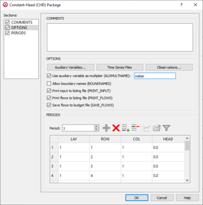
The Constant-Head (CHD) Package dialog is accessed by double-clicking on the CHD package under a MODFLOW 6 simulation in the Project Explorer. It contains the following sections and options:
- Sections list – A list of sections that can be turned on or off:
- Comments – Turn on to make the Comments section visible.
- Options – Turn on to make the Options section visible.
- Periods – Turn on to make the Periods section visible. This section is on by default.
- Comments section – Enter general alphanumeric comments. Comments entered here get written at the top of the file, preceded by a '#' symbol.
- Options section – Contains the following:
- Auxiliary Variables... – Click to bring up the Auxiliary Variables dialog.
- Time Series... – Click to bring up the Time Series Files dialog.
- Observations... – Click to bring up the Observation Files dialog.
- Use auxiliary variable as multiplier (AUXMULTNAME) – Name of auxiliary variable to be used as multiplier of CHD head value.
- Allow boundary names (BOUNDNAMES) – Turn on to allow boundary names to be included in the list of constant-head cells.
- Print input to listing file (PRINT_INPUT) – Turn on to write the list of constant-head information to the listing file immediately after it is read.
- Print flows to listing file (PRINT_FLOWS) – Turn on to write the list of constant-head flow rates to the listing file for every stress period time step in which "BUDGET PRINT" is specified in Output Control.
- Save flows to budget file (SAVE_FLOWS) – Turn on to write constant-head flow terms to the file specified with "BUDGET FILEOUT" in Output Control.
- Use with Water Mover (MVR) package (MOVER) – Turn on to allows this instance of the Constant-Head Package to be used with the Water Mover (MVR) Package.
- Periods section – Contains the following:
- Period drop-down – Use the Increment Up and Down
 buttons to select the desired period.
 - Define Period
 – If no period is defined, click to make the spreadsheet editable.
 - Delete Period
 – Click to delete the existing period.
 - Add Rows
 – Click to bring up the Add Stresses dialog.
 - Delete Rows
 – Click to bring up a dialog with three options:
- Delete from All Periods – Click to delete matching stresses from all periods.
- Delete from Just This Period – Click to delete matching stresses from just this period.
- Cancel – Click to close the dialog without deleting anything.
- Plot All Periods
 – Click to bring up the XY Series Editor dialog.
 - Open Time Series
 – Click to bring up the
 - Filter on Selected Cells
 – Click to turn on filtering on the selected cells.
- Period drop-down – Use the Increment Up and Down
Drain (DRN) Package
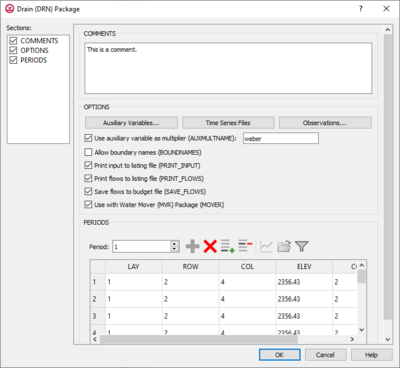
The Drain (DRN) Package dialog is accessed by double-clicking on the DRN package under a MODFLOW 6 simulation in the Project Explorer. It contains the following sections and options:
- Sections list – A list of sections that can be turned on or off:
- Comments – Turn on to make the Comments section visible.
- Options – Turn on to make the Options section visible.
- Periods – Turn on to make the Periods section visible. This section is on by default.
- Comments section – Enter general alphanumeric comments. Comments entered here get written at the top of the file, preceded by a '#' symbol.
- Options section
- Auxiliary Variables... – Click to bring up the Auxiliary Variables dialog.
- Time Series... – Click to bring up the Time Series Files dialog.
- Observations... – Click to bring up the Observation Files dialog.
- Use auxiliary variable as multiplier (AUXMULTNAME) – Name of auxiliary variable to be used as multiplier of drain conductance.
- Allow boundary names (BOUNDNAMES) – Turn on to allow boundary names to be included in the list of drain cells.
- Print input to listing file (PRINT_INPUT) – Turn on to write the list of drain information to the listing file immediately after it is read.
- Print flows to listing file (PRINT_FLOWS) – Turn on to write the list of drain flow rates to the listing file for every stress period time step in which "BUDGET PRINT" is specified in Output Control.
- Save flows to budget file (SAVE_FLOWS) – Turn on to write drain flow terms to the file specified with "BUDGET FILEOUT" in Output Control.
- Use with Water Mover (MVR) package (MOVER) – Turn on to allows this instance of the Drain Package to be used with the Water Mover (MVR) Package.
- Periods section – Contains the following:
- Period drop-down – Use the Increment Up and Down
 buttons to select the desired period.
 - Define Period
 – If no period is defined, click to make the spreadsheet editable.
 - Delete Period
 – Click to delete the existing period.
 - Add Rows
 – Click to bring up the Add Stresses dialog.
 - Delete Rows
 – Click to bring up a dialog with three options:
- Delete from All Periods – Click to delete matching stresses from all periods.
- Delete from Just This Period – Click to delete matching stresses from just this period.
- Cancel – Click to close the dialog without deleting anything.
- Plot All Periods
 – Click to bring up the XY Series Editor dialog.
 - Open Time Series
 – Click to bring up the
 - Filter on Selected Cells
 – Click to turn on filtering on the selected cells.
- Period drop-down – Use the Increment Up and Down
EVT
GHB
GNC
HFB
LAK
MAW
MVR
OBS
OC
RCH
RIV
SFR
STO
UZF
WEL
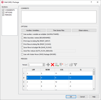
The Well (WEL) Package dialog is accessed by double-clicking on the WEL package under a MODFLOW 6 simulation in the Project Explorer. It contains the following sections and options:
- Sections list – A list of sections that can be turned on or off:
- Comments – Turn on to make the Comments section visible.
- Options – Turn on to make the Options section visible.
- Periods – Turn on to make the Periods section visible.
- Comments section – Enter general alphanumeric comments. Comments entered here get written at the top of the file, preceded by a '#' symbol.
- Options section – Temporal options and settings:
- Auxiliary Variables... – Click to bring up the Auxiliary Variables dialog.
- Time Series... – Click to bring up the Time Series Files dialog.
- Observations... – Click to bring up the Observation Files dialog.
- Use auxiliary variable as multiplier (AUXMULTNAME) – Name of auxiliary variable to be used as multiplier of drain conductance.
- Allow boundary names (BOUNDNAMES) – Turn on to allow boundary names to be included in the list of drain cells.
- Print input to listing file (PRINT_INPUT) – Turn on to write the list of drain information to the listing file immediately after it is read.
- Print flows to listing file (PRINT_FLOWS) – Turn on to write the list of drain flow rates to the listing file for every stress period time step in which "BUDGET PRINT" is specified in Output Control.
- Save flows to budget file (SAVE_FLOWS) – Turn on to write drain flow terms to the file specified with "BUDGET FILEOUT" in Output Control.
- Use with Water Mover (MVR) package (MOVER) – Turn on to allows this instance of the Drain Package to be used with the Water Mover (MVR) Package.
- Periods section – Contains the following:
- Period drop-down – Use the Increment Up and Down
 buttons to select the desired period.
 - Define Period
 – If no period is defined, click to make the spreadsheet editable.
 - Delete Period
 – Click to delete the existing period.
 - Add Rows
 – Click to bring up the Add Stresses dialog.
 - Delete Rows
 – Click to bring up a dialog with three options:
- Delete from All Periods – Click to delete matching stresses from all periods.
- Delete from Just This Period – Click to delete matching stresses from just this period.
- Cancel – Click to close the dialog without deleting anything.
- Plot All Periods
 – Click to bring up the XY Series Editor dialog.
 - Open Time Series
 – Click to bring up the
 - Filter on Selected Cells
 – Click to turn on filtering on the selected cells.
- Period drop-down – Use the Increment Up and Down
ZONE FILE
Date/Time Dialog
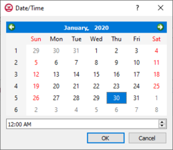
The Date/Time dialog allows setting the date and time for a number of different options through selecting the desired date from a calendar:
- The
 Left and
  Right arrows allow the user to change to one month earlier or later (respectively).
 - The month name at the top of the calendar is a drop-down menu allowing the user to select the desired month.
- The year at the top of the calendar allows the year to be changed up or down using the
 Increment Up/Down buttons.
 - The time is either manually entered in "HH:MM AM/PM" format, or selected using the
 Increment Up/Down buttons.
The following buttons are found at bottom of the dialog:
- OK – Saves all changes and closes the Date/Time dialog.
- Cancel – Discards all changes and closes the Date/Time dialog.
Auxiliary Variables Dialog
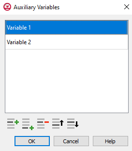
The Auxiliary Variables dialog is accessed by clicking Auxiliary Variables... in the Options section of the Constant-Head (CHD) Package dialog. It is used to define an array of one or more auxiliary variable names. It contains the following options:
Time Series Files Dialog
The Time Series Files dialog is accessed by clicking Time Series Files... in the Options section of the Constant-Head (CHD) Package dialog. It contains the following options:
Observation Files Dialog
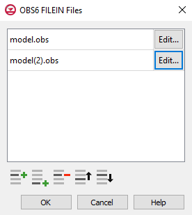
The Observation Files dialog is accessed by clicking Observations... in the Options section of the Constant-Head (CHD) Package dialog. It contains the following options:
Add Stresses Dialog
The Add Stresses dialog is accessed by clicking Add Rows ![]() in the Periods section of the Constant-Head (CHD) Package dialog. It contains the following sections and options:
in the Periods section of the Constant-Head (CHD) Package dialog. It contains the following sections and options:
- LAY – Enter an integer in the Value column on this row equal to the layer number for the row(s) being added.
- ROW – Enter an integer in the Value column on this row equal to the row number for the row(s) being added.
- LAY – Enter an integer in the Value column on this row equal to the column number for the row(s) being added.
- HEAD – Enter a decimal value of the head for the row(s) being added.
- Number of rows to add – Use the Increment Up and Down
 buttons to select the desired number of rows to add.
 - Add to section – Radio buttons with the following options:
- All defined periods – Select to add the rows to all defined periods.
- Only this period – Select to add the rows to only this period.
External Link
| GMS – Groundwater Modeling System | ||
|---|---|---|
| Modules: | 2D Grid • 2D Mesh • 2D Scatter Point • 3D Grid • 3D Mesh • 3D Scatter Point • Boreholes • GIS • Map • Solid • TINs • UGrids | |
| Models: | FEFLOW • FEMWATER • HydroGeoSphere • MODAEM • MODFLOW • MODPATH • mod-PATH3DU • MT3DMS • MT3D-USGS • PEST • PHT3D • RT3D • SEAM3D • SEAWAT • SEEP2D • T-PROGS • ZONEBUDGET | |
| Aquaveo | ||
