User:Jcreer/MODFLOW 6 Changes for GMS 10.6: Difference between revisions
(→RCH) |
(→RCH) |
||
| Line 537: | Line 537: | ||
*''Comments'' section – Enter general alphanumeric comments. Comments entered here get written at the top of the file, preceded by a '#' symbol. | *''Comments'' section – Enter general alphanumeric comments. Comments entered here get written at the top of the file, preceded by a '#' symbol. | ||
*''Options'' section – Temporal options and settings: | *''Options'' section – Temporal options and settings: | ||
**'''Auxiliary Variables...''' | **''AUXILIARY'' – Click the '''Auxiliary Variables...''' button to bring up the [[#Auxiliary Variables Dialog|''Auxiliary Variables'' dialog]]. | ||
**'''Time-Array Series Files''' – Click to bring up the [[#Time-Array Series Files Dialog|''Time-Array Series Files'' dialog]]. | **'''Time-Array Series Files''' – Click to bring up the [[#Time-Array Series Files Dialog|''Time-Array Series Files'' dialog]]. | ||
**'''Observations...''' – Click to bring up the [[#Observation Files Dialog|''Observation Files'' dialog]]. | **'''Observations...''' – Click to bring up the [[#Observation Files Dialog|''Observation Files'' dialog]]. | ||
Revision as of 23:08, 24 August 2021
| This contains information about functionality available starting at GMS version 10.6. The content may not apply to other versions. |
Contents
Package Updates
TDIS
| MODFLOW 6 is currently in Beta release for GMS Some features and capabilities of MODFLOW 6 are still in development for GMS. |
| MODFLOW 6 | |
|---|---|
| Models & Tools | |
|
GWF Model GWT Model Cell Properties Dialog Zone File | |
| Packages | |
| Flow: | GNC, HFB, NPF |
| GWF: |
BUY, CHD, CSUB, DRN, EVT, GHB, LAK, MAW, MVR, OBS, RCH,RIV, SFR, STO, UZF, WEL |
| GWT: |
ADV, CNC, DSP FMI, IC, IST, LKT, MDT, MST, MVT, MWT, OBS, SFT, SRC,SSM, UZT |
| Other |
DIS, DISU, DISV, IMS, OC, TDIS, PEST |
The Temporal Discretization (TDIS) Package dialog is accessed by double-clicking on the TDIS package under a MODFLOW 6 simulation in the Project Explorer. It contains the following sections and options:
- Sections list – A list of sections that can be turned on or off:
- Comments – Turn on to make the Comments section visible.
- Options – Turn on to make the Options section visible.
- PeriodData – Turn on to make the PeriodData section visible. This section is on by default.
- Comments section – Enter general alphanumeric comments. Comments entered here get written at the top of the file, preceded by a '#' symbol.
- Options section – Temporal options and settings:
- Time units drop-down – Time unit label used in output files. Contains a drop-down menu with the following options for the type of time units:
- "Unknown"
- "Seconds"
- "Minutes"
- "Hours"
- "Days" – The default selection.
- "Years"
- Start date/time – Starting date and time. Turn on to enable setting a start date/time. Included in the list file using the selected time/date. Click the Date/Time... button to bring up the Date/Time dialog. The time can also be manually entered using "YYYY-MM-DDTHH:MM:SS" format. The "T" in the middle divides the date from the time.
- Time units drop-down – Time unit label used in output files. Contains a drop-down menu with the following options for the type of time units:
- PeriodData section – Contains a spreadsheet listing periods. An
 Add Row button is found at the top rigth of the spreadsheet. Right-clicking on the row number in the spreadsheet gives a menu that allows inserting, deleting, copying, or pasting a row. The columns in the spreadsheet include:
- PERLEN – The length of a stress period. The default value is "1.0".
- NSTP – The number of time steps in a stress period. The default value is "1".
- TSMULT – The multiplier for the length of successive time steps. The default value is "1.0".
- ENDDATE – The end date for that period. This field is not directly user-editable, but will automatically change if the PERLEN value is changed.
- STEADY-STATE GWF_Model – Turn on if the period is steady state and using the GWF Model.
CHD
| MODFLOW 6 | |
|---|---|
| Models & Tools | |
|
GWF Model GWT Model Cell Properties Dialog Zone File | |
| Packages | |
| Flow: | GNC, HFB, NPF |
| GWF: |
BUY, CHD, CSUB, DRN, EVT, GHB, LAK, MAW, MVR, OBS, RCH,RIV, SFR, STO, UZF, WEL |
| GWT: |
ADV, CNC, DSP FMI, IC, IST, LKT, MDT, MST, MVT, MWT, OBS, SFT, SRC,SSM, UZT |
| Other |
DIS, DISU, DISV, IMS, OC, TDIS, PEST |
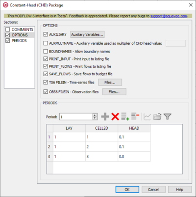
The Constant-Head (CHD) Package dialog is accessed by double-clicking on the CHD package under a MODFLOW 6 simulation in the Project Explorer. It contains the following sections and options:
- Sections list – A list of sections that can be turned on or off:
- Comments – Turn on to make the Comments section visible.
- Options – Turn on to make the Options section visible.
- Periods – Turn on to make the Periods section visible. This section is on by default.
- Comments section – Enter general alphanumeric comments. Comments entered here get written at the top of the file, preceded by a '#' symbol.
- Options section – Contains the following:
- AUXILIARY – Click the Auxiliary Variables... button to bring up the Auxiliary Variables dialog.
- AUXMULTNAME – Auxiliary variable used as multiplier of CHD head value. Enter the name of auxiliary variable to be used as multiplier of CHD head value.
- BOUNDNAMES – Allow boundary names. Turn on to allow boundary names to be included in the list of constant-head cells.
- PRINT_INPUT – Print input to listing file. Turn on to write the list of constant-head information to the listing file immediately after it is read.
- PRINT_FLOWS – Print flows to listing file. Turn on to write the list of constant-head flow rates to the listing file for every stress period time step in which "BUDGET PRINT" is specified in Output Control.
- SAVE_FLOWS – Save flows to budget file. Turn on to write constant-head flow terms to the file specified with "BUDGET FILEOUT" in Output Control.
- TS6 FILEIN – Define time series files. Click the Files... button to bring up the Time Series Files dialog.
- OBS6 FILEIN – Define observation files. Click the Files... button to bring up the Observation Files dialog.
- Periods section – Contains the following:
- Period value – Use the Increment Up and Down
 buttons to select the desired period.
 - Define Period
 – If no period is defined, click to make the spreadsheet editable.
 - Delete Period
 – Click to delete the existing period.
 - Add Rows
 – Click to bring up the Add Stresses dialog.
 - Delete Rows
 – Click to bring up a dialog with three options:
- Delete from All Periods – Click to delete matching stresses from all periods.
- Delete from Just This Period – Click to delete matching stresses from just this period.
- Plot All Periods
 – Click to bring up the XY Series Editor dialog. Requires that a cell be selected in the table.
 - Open Time Series
 – Click to bring up the
 - Filter on Selected Cells
 – Click to turn on filtering on the selected cells.
- Table – Contains the following:
- LAY – Used to specify which layer is being applied.
- CELL2D – Enter the cell ID that is being applied.
- HEAD – Represents the head at the boundary.
- Table – Contains the following:
- Period value – Use the Increment Up and Down
DRN
| MODFLOW 6 | |
|---|---|
| Models & Tools | |
|
GWF Model GWT Model Cell Properties Dialog Zone File | |
| Packages | |
| Flow: | GNC, HFB, NPF |
| GWF: |
BUY, CHD, CSUB, DRN, EVT, GHB, LAK, MAW, MVR, OBS, RCH,RIV, SFR, STO, UZF, WEL |
| GWT: |
ADV, CNC, DSP FMI, IC, IST, LKT, MDT, MST, MVT, MWT, OBS, SFT, SRC,SSM, UZT |
| Other |
DIS, DISU, DISV, IMS, OC, TDIS, PEST |
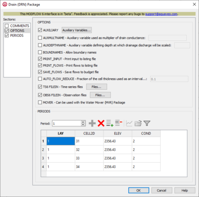
The Drain (DRN) Package dialog is accessed by double-clicking on the DRN package under a MODFLOW 6 simulation in the Project Explorer. It contains the following sections and options:
- Sections list – A list of sections that can be turned on or off:
- Comments – Turn on to make the Comments section visible.
- Options – Turn on to make the Options section visible.
- Periods – Turn on to make the Periods section visible. This section is on by default.
- Comments section – Enter general alphanumeric comments. Comments entered here get written at the top of the file, preceded by a '#' symbol.
- Options section
- AUXILIARY – Click the Auxiliary Variables... button to bring up the Auxiliary Variables dialog.
- AUXMULTNAME – Auxiliary variable used as multiplier of drain conductance. Enter the name of auxiliary variable to be used as multiplier of drain conductance.
- AUXDEPTHNAME – Auxiliary variable defining depth at which drainage discharge will be scaled.
- BOUNDNAMES – Allow boundary names. Turn on to allow boundary names to be included in the list of drain cells.
- PRINT_INPUT – Print input to listing file. Turn on to write the list of drain conductance information to the listing file immediately after it is read.
- PRINT_FLOWS – Print flows to listing file. Turn on to write the list of drain conductance rates to the listing file for every stress period time step in which "BUDGET PRINT" is specified in Output Control.
- TS6 FILEIN – Define time series files. Click the Files... button to bring up the Time Series Files dialog.
- OBS6 FILEIN – Define observation files. Click the Files... button to bring up the Observation Files dialog.
- MOVER – Can be used with the Water Mover (MVR) package. Turn on to allows this instance of the Drain Package to be used with the Water Mover (MVR) Package.
- Periods section – Contains the following:
- Period drop-down – Use the Increment Up and Down
 buttons to select the desired period.
 - Define Period
 – If no period is defined, click to make the spreadsheet editable.
 - Delete Period
 – Click to delete the existing period.
 - Add Rows
 – Click to bring up the Add Stresses dialog.
 - Delete Rows
 – Click to bring up a dialog with three options:
- Delete from All Periods – Click to delete matching stresses from all periods.
- Delete from Just This Period – Click to delete matching stresses from just this period.
- Plot All Periods
 – Click to bring up the XY Series Editor dialog. Requires that a cell be selected in the table.
 - Open Time Series
 – Click to bring up the
 - Filter on Selected Cells
 – Click to turn on filtering on the selected cells.
- Table – Contains the following:
- LAY – Used to specify which layer is being applied.
- CELL2D – Enter the cell ID that is being applied.
- ELEV – Represents the elevation of the drain.
- COND – Represents the hydraulic conductance between the aquifer and the drain.
- Table – Contains the following:
- Period drop-down – Use the Increment Up and Down
EVT
| MODFLOW 6 | |
|---|---|
| Models & Tools | |
|
GWF Model GWT Model Cell Properties Dialog Zone File | |
| Packages | |
| Flow: | GNC, HFB, NPF |
| GWF: |
BUY, CHD, CSUB, DRN, EVT, GHB, LAK, MAW, MVR, OBS, RCH,RIV, SFR, STO, UZF, WEL |
| GWT: |
ADV, CNC, DSP FMI, IC, IST, LKT, MDT, MST, MVT, MWT, OBS, SFT, SRC,SSM, UZT |
| Other |
DIS, DISU, DISV, IMS, OC, TDIS, PEST |
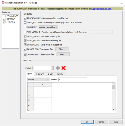
The Evapotranspiration (EVT) Package dialog is accessed by double-clicking on the EVT package under a MODFLOW 6 simulation in the Project Explorer. It contains the following sections and options:
- Sections list – A list of sections that can be turned on or off:
- Comments – Turn on to make the Comments section visible.
- Options – Turn on to make the Options section visible.
- PeriodData – Turn on to make the PeriodData section visible. This section is on by default.
- Comments section – Enter general alphanumeric comments. Comments entered here get written at the top of the file, preceded by a '#' symbol.
- Options section – Temporal options and settings:
- READASARRAYS – Array-baseed input with be used. Select to specify to use array-based input in the EVT package.
- FIXED_CELL – Do not reassign to underlying cell if cell is inactive. Turn on to indicate that evapotranspiration will not be reassigned to a cell underlying the cell specified in the list if the specified cell is inactive.
- AUXILIARY – Click the Auxiliary Variables... button to bring up the Auxiliary Variables dialog.
- AUXMULTNAME – Auxiliary variable used as multiplier of evapotranspiration rate. Enter the name of auxiliary variable to be used as multiplier of evapotranspiration rate.
- BOUNDNAMES – Allow boundary names. Turn on to allow boundary names to be included in the list of evapotranspiration cells.
- PRINT_INPUT – Print input to listing file. Turn on to write the list of evapotranspiration rates to the listing file immediately after it is read.
- PRINT_FLOWS – Print flows to listing file. Turn on to write the list of evapotranspiration rates to the listing file for every stress period time step in which "BUDGET PRINT" is specified in Output Control.
- SAVE_FLOWS – Save flows to budget file. Turn on to write evapotranspiration terms to the file specified with "BUDGET FILEOUT" in Output Control.
- TS6 FILEIN – Define time series files. Click the Files... button to bring up the Time Series Files dialog.
- OBS6 FILEIN – Define observation files. Click the Files... button to bring up the Observation Files dialog
- Periods section – Contains the following:
- Table – Contains four tabs:
- IEVT – The layer number that defines the layer in each vertical column.
- "UNDEFINED" – Indicates that there are no definite variables to be applied.
- "CONSTANT" – If "Constant" is selected from the drop-down, enter a decimal value in the Constant field to be applied to all cells in the layer(s).
- "ARRAY" – If "Array" is selected from the drop-down, enter an integer in the factor: field to be multiplied to the array after it is read.
- "TIME-ARRAY SERIES" – Is not supported for IEVT, SURFACE, or DEPTH.
- SURFACE – The elevation of the ET surface.
- "UNDEFINED" – Indicates that there are no definite variable to be applied.
- "CONSTANT" – If "Constant" is selected from the drop-down, enter a decimal value in the Constant field to be applied to all cells in the layer(s).
- "ARRAY" – If "Array" is selected from the drop-down, enter an integer in the factor: field to be multiplied to the array after it is read.
- "TIME-ARRAY SERIES" – Is not supported for IEVT, SURFACE, or DEPTH.
- RATE – The maximum ET flux rate.
- "UNDEFINED" – Indicates that there are no definite variables to be applied.
- "CONSTANT" – If "Constant" is selected from the drop-down, enter a decimal value in the Constant field to be applied to all cells in the layer(s).
- "ARRAY" – If "Array" is selected from the drop-down, enter an integer in the factor: field to be multiplied to the array after it is read.
- "TIME-ARRAY SERIES" – If "Time-Array Series" is selected from the drop-down, indicate which Time-Array Series is being applied in the Series: field.
- DEPTH – The ET extinction depth.
- "UNDEFINED" – Indicates that there are no definite variable to be applied.
- "CONSTANT" – If "Constant" is selected from the drop-down, enter a decimal value in the Constant field to be applied to all cells in the layer(s).
- "ARRAY" – If "Array" is selected from the drop-down, enter an integer in the factor: field to be multiplied to the array after it is read.
- "TIME-ARRAY SERIES" – Is not supported for IEVT, SURFACE, or DEPTH.
- IEVT – The layer number that defines the layer in each vertical column.
GHB
| MODFLOW 6 | |
|---|---|
| Models & Tools | |
|
GWF Model GWT Model Cell Properties Dialog Zone File | |
| Packages | |
| Flow: | GNC, HFB, NPF |
| GWF: |
BUY, CHD, CSUB, DRN, EVT, GHB, LAK, MAW, MVR, OBS, RCH,RIV, SFR, STO, UZF, WEL |
| GWT: |
ADV, CNC, DSP FMI, IC, IST, LKT, MDT, MST, MVT, MWT, OBS, SFT, SRC,SSM, UZT |
| Other |
DIS, DISU, DISV, IMS, OC, TDIS, PEST |
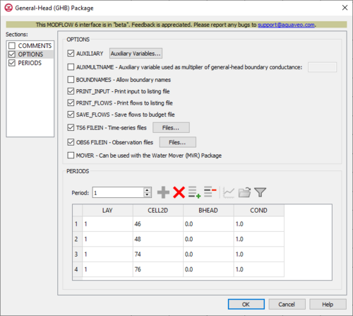
The General-Head (GHB) Package dialog is accessed by double-clicking on the GHB package under a MODFLOW 6 simulation in the Project Explorer. It contains the following sections and options:
- Sections list – A list of sections that can be turned on or off:
- Comments – Turn on to make the Comments section visible.
- Options – Turn on to make the Options section visible.
- Periods – Turn on to make the Periods section visible. This section is on by default.
- Comments section – Enter general alphanumeric comments. Comments entered here get written at the top of the file, preceded by a '#' symbol.
- Options section – Contains the following:
- AUXILIARY – Click the Auxiliary Variables... button to bring up the Auxiliary Variables dialog.
- AUXMULTNAME – Auxiliary variable used as multiplier of general head value. Enter the name of auxiliary variable to be used as multiplier of general head value.
- BOUNDNAMES – Allow boundary names. Turn on to allow boundary names to be included in the list of general head cells.
- PRINT_INPUT – Print input to listing file. Turn on to write the list of general head information to the listing file immediately after it is read.
- PRINT_FLOWS – Print flows to listing file. Turn on to write the list of general head flow rates to the listing file for every stress period time step in which "BUDGET PRINT" is specified in Output Control.
- SAVE_FLOWS – Save flows to budget file. Turn on to write general head flow terms to the file specified with "BUDGET FILEOUT" in Output Control.
- TS6 FILEIN – Define time series files. Click the Files... button to bring up the Time Series Files dialog.
- OBS6 FILEIN – Define observation files. Click teh Files... button to bring up the Observation Files dialog.
- MOVER – Can be used with the Water Mover (MVR) package. Turn on to allows this instance of the General-Head Package to be used with the Water Mover (MVR) Package.
- Periods section – Contains the following:
- Period drop-down – Use the Increment Up and Down
 buttons to select the desired period.
 - Define Period
 – If no period is defined, click to make the spreadsheet editable.
 - Delete Period
 – Click to delete the existing period.
 - Add Rows
 – Click to bring up the Add Stresses dialog.
 - Delete Rows
 – Click to bring up a dialog with three options:
- Delete from All Periods – Click to delete matching stresses from all periods.
- Delete from Just This Period – Click to delete matching stresses from just this period.
- Plot All Periods
 – Click to bring up the XY Series Editor dialog. Requires that a cell be selected in the table.
 - Open Time Series
 – Click to bring up the
 - Filter on Selected Cells
 – Click to turn on filtering on the selected cells.
 - Table – Contains the following:
- LAY – Used to specify which layer is being applied.
- CELL2D – Enter the cell ID that is being applied.
- BHEAD – Represents the boundary head.
- COND – Represents the hydraulic conductance between the aquifer cell and the boundary.
- Period drop-down – Use the Increment Up and Down
GNC
HFB
| MODFLOW 6 | |
|---|---|
| Models & Tools | |
|
GWF Model GWT Model Cell Properties Dialog Zone File | |
| Packages | |
| Flow: | GNC, HFB, NPF |
| GWF: |
BUY, CHD, CSUB, DRN, EVT, GHB, LAK, MAW, MVR, OBS, RCH,RIV, SFR, STO, UZF, WEL |
| GWT: |
ADV, CNC, DSP FMI, IC, IST, LKT, MDT, MST, MVT, MWT, OBS, SFT, SRC,SSM, UZT |
| Other |
DIS, DISU, DISV, IMS, OC, TDIS, PEST |
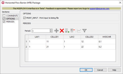
The Horizontal Flow Barrier (HFB) Package dialog is accessed by double-clicking on the HFB package under a MODFLOW 6 simulation in the Project Explorer. It contains the following sections and options:
- Sections list – A list of sections that can be turned on or off:
- Comments – Turn on to make the Comments section visible.
- Options – Turn on to make the Options section visible.
- Periods – Turn on to make the Periods section visible. This section is on by default.
- Comments section – Enter general alphanumeric comments. Comments entered here get written at the top of the file, preceded by a '#' symbol.
- Options section – Temporal options and settings:
- PRINT_INPUT – Print input to listing file. Turn on to write the list of flow barrier information to the listing file immediately after it is read.
- Periods section – Contains the following:
- Period drop-down – Use the Increment Up and Down
 buttons to select the desired period.
 - Define Period
 – If no period is defined, click to make the spreadsheet editable.
 - Delete Period
 – Click to delete the existing period.
 - Add Rows
 – Click to bring up the Add Stresses dialog.
 - Delete Rows
 – Click to bring up a dialog with three options:
- Delete from All Periods – Click to delete matching stresses from all periods.
- Delete from Just This Period – Click to delete matching stresses from just this period.
- Plot All Periods
 – Click to bring up the XY Series Editor dialog. Requires that a cell be selected in the table.
 - Open Time Series
 – Click to bring up the
 - Filter on Selected Cells
 – Click to turn on filtering on the selected cells.
 - Table – Contains the following:
- LAY1 – Identifier for the first layer.
- CELL2D1 – Enter the cell ID that is being applied to the first layer.
- LAY2 – Identifier for the second layer.
- CELL2D2 – Enter the cell ID that is being applied to the second layer.
- HYDCHR – The hydraulic characteristic of the horizontal-flow barrier. When this variable is negative it multiplied by the conductance of two cells.
- Period drop-down – Use the Increment Up and Down
LAK
| MODFLOW 6 | |
|---|---|
| Models & Tools | |
|
GWF Model GWT Model Cell Properties Dialog Zone File | |
| Packages | |
| Flow: | GNC, HFB, NPF |
| GWF: |
BUY, CHD, CSUB, DRN, EVT, GHB, LAK, MAW, MVR, OBS, RCH,RIV, SFR, STO, UZF, WEL |
| GWT: |
ADV, CNC, DSP FMI, IC, IST, LKT, MDT, MST, MVT, MWT, OBS, SFT, SRC,SSM, UZT |
| Other |
DIS, DISU, DISV, IMS, OC, TDIS, PEST |
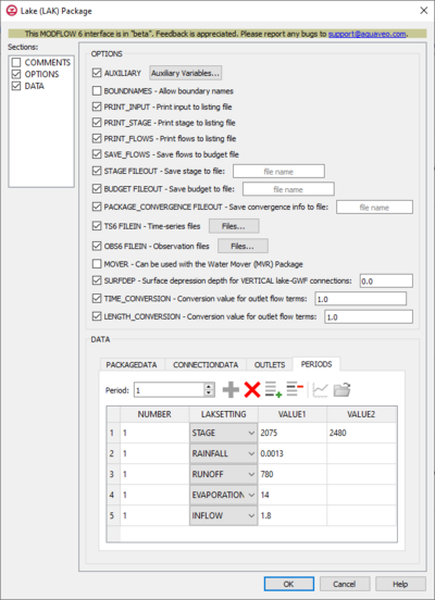
The Lake (LAK) Package dialog is accessed by double-clicking on the WEL package under a MODFLOW 6 simulation in the Project Explorer. It contains the following sections and options:
- Sections list – A list of sections that can be turned on or off:
- Comments – Turn on to make the Comments section visible.
- Options – Turn on to make the Options section visible.
- Data – Turn on to make the Data section visible. This section is on by default.
- Comments section – Enter general alphanumeric comments. Comments entered here get written at the top of the file, preceded by a '#' symbol.
- Options section – Temporal options and settings:
- AUXILIARY – Click the Auxiliary Variables... button to bring up the Auxiliary Variables dialog.
- BOUNDNAMES – Allow boundary names. If turned on, indicates that the list of lake cells will be provided with the associative boundary names.
- PRINT_INPUT – Print input to listing file. If turned on, indicates that the list of lake information will be written to the listing file after it is read.
- PRINT_STAGE – Print stage to listing file. If turned on, indicates that lake stages will be printed to the listing file for each stress period if "HEAD PRINT" is specified.
- PRINT_FLOWS – Print flows to listing file. If turned on, indicates that a list of lake flow rates will be printed to the listing file.
- SAVE_FLOWS – Save flows to budget file. If turned on, indicates that the lake flow terms will be written to a specified file.
- STAGE_FILEOUT – Save stage to file. Indicates that the record corresponds to a specific stage. Also allows the written indication of stage information.
- BUDGET_FILEOUT – Save budget to file. Allows the specification of a file to which desired flow terms will be written.
- PACKAGE_CONVERGNECE FILEOUT – Save convergence info to file.
- TS6 FILEIN – Define time series files. Click the Files... button to bring up the Time Series Files dialog.
- OBS6 FILEIN – Define observation files. Click the Files... button to bring up the Observation Files dialog.
- MOVER – When turned on, indicates that the Lake (Lak) Package, in this instance can be used in collaboration with the Water Mover (MVR) Package.
- SURFDEP – When turned on, allows the a written value that defines the surface depression depth of the lake.
- TIME_CONVERSION – Value that is used in converting outlet flow terms into time units.
- LENGTH_CONVERSION – Value that is used in converting outlet flow terms into length units.
- Data section – Contains the following:
- PackageData
- Add Rows – Click to bring up the Rows to Add dialog where the number of rows to add to the bottom can be specified.
- LAKENO
- STRT
- NLAKECONN
- ConnectionData
- Add Rows – Click to bring up the Rows to Add dialog where the number of rows to add to the bottom can be specified.
- LAKENO
- ICONN
- LAY
- CELL2D
- CLAKTYPE
- BELEAK
- BELEV
- TELEV
- CONNLEN
- CONNWIDTH
- Outlets
- Add Rows – Click to bring up the Rows to Add dialog where the number of rows to add to the bottom can be specified.
- OUTLETNO – The outlet number.
- LAKEIN –
- LAKEOUT –
- COUTTYPE – Defines which of three outlet types applies to the current outlet.
- "Specified"
- "Manning"
- "Weir"
- INVERT – The invert elevation for the lake outlet.
- WIDTH – The width of the lake outlet.
- ROUGH – The roughness coefficient for the lake outlet.
- SLOPE – The bed slope for the lake outlet.
- Periods tab
- Periods drop-down – Use the Increment Up and Down
 buttons to select the desired period.
 - Define Period
 – If no period is defined, click to make the spreadsheet editable.
 - Delete Period
 – Click to delete the existing period.
 - Add Rows
 – Click to bring up the Add Stresses dialog.
 - Delete Rows
 – Click to bring up a dialog with three options:
- Delete from All Periods – Click to delete matching stresses from all periods.
- Delete from Just This Period – Click to delete matching stresses from just this period.
- Plot All Periods
 – Click to bring up the XY Series Editor dialog. Requires that a cell be selected in the table.
 - Open Time Series
 – Click to bring up the
 - Filter on Selected Cells
 – Click to turn on filtering on the selected cells.
 - Table – Allows the manual input of different variables for the MAW Package.
- NUMBER – A value that defines the reach number associated with the specified PERIOD data.
- LAKSETTING – Information that is linked to keywords and values.
- VALUE1 – Value to be entered in relation to the specific project.
- VALUE2 – Value to be entered in relation to the specific project.
- Periods drop-down – Use the Increment Up and Down
- PackageData
MAW
| MODFLOW 6 | |
|---|---|
| Models & Tools | |
|
GWF Model GWT Model Cell Properties Dialog Zone File | |
| Packages | |
| Flow: | GNC, HFB, NPF |
| GWF: |
BUY, CHD, CSUB, DRN, EVT, GHB, LAK, MAW, MVR, OBS, RCH,RIV, SFR, STO, UZF, WEL |
| GWT: |
ADV, CNC, DSP FMI, IC, IST, LKT, MDT, MST, MVT, MWT, OBS, SFT, SRC,SSM, UZT |
| Other |
DIS, DISU, DISV, IMS, OC, TDIS, PEST |
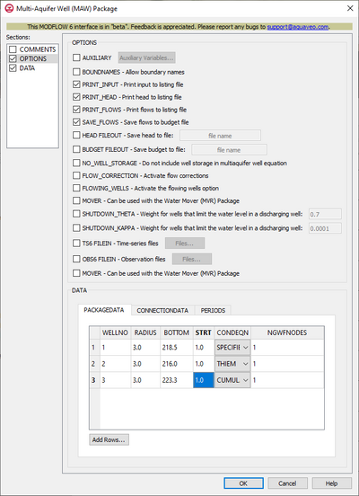
The Multi-Aquifer Well (MAW) Package dialog is accessed by double-clicking on the WEL package under a MODFLOW 6 simulation in the Project Explorer. It contains the following sections and options:
- Sections list – A list of sections that can be turned on or off:
- Comments – Turn on to make the Comments section visible.
- Options – Turn on to make the Options section visible.
- Data – Turn on to make the Data section visible. This section is on by default.
- Comments section – Enter general alphanumeric comments. Comments entered here get written at the top of the file, preceded by a '#' symbol.
- Options section – Temporal options and settings:
- AUXILIARY – Click the Auxiliary Variables... button to bring up the Auxiliary Variables dialog.
- BOUNDNAMES – Allow boundary names. If turned on, indicates that the list of multi-aquifer well cells will be provided with the associative boundary names.
- PRINT_INPUT – Print input to listing file. Print input to listing file. If turned on, indicates that the list of multi-aquifer well information will be written to the listing file after it is read.
- PRINT_HEAD – Print head to listing file. If turned on, indicates that well heads will be printed to the listing file for each stress period that "HEAD PRINT" is specified.
- PRINT_FLOWS – Print flows to listing file. If turned on, indicates that a list of multi-aquifer well flow rates will be printed to the listing file.
- SAVE_FLOWS – Saves flow to budget file. If turned on, indicates that the multi-aquifer well flow terms will be written to a specified file.
- HEAD_FILEOUT – Save head to file. Enter the name of the output file to write stage information.
- BUDGET_FILEOUT – Save budget to file. Allows the specification of a file to which desired flow terms will be written.
- NO_WELL_STORAGE – If turned on, indicates that well storage will not be included in the continuity equation. It is used to control discharge rate oscillations.
- FLOW_CORRECTION – Activate flow corrections.
- FLOWING_WELLS – If turned on, indicates that the flowing wells option is activated.
- MOVER – When turned on, indicates that the Multi-Aquifer Well (MAW) Package, in this instance can be used in collaboration with the Water Mover (MVR) Package.
- SHUTDOWN_THETA – Defines the weight that is applied to the discharge rate for wells that have water limitations.
- SHUTDOWN_KAPPA – Defines the weight that is applied to the discharge rate for wells that have water limitations. It is used to control discharge rate oscillations.
- TS6 FILEIN – Define time series files. Click the Files... button to bring up the Time Series Files dialog.
- OBS6 FILEIN – Define observation files. Click the Files... button to bring up the Observation Files dialog.
- Data section – Contains the following:
- Periods drop-down – Use the Increment Up and Down
 buttons to select the desired period.
 - Define Period
 – If no period is defined, click to make the spreadsheet editable.
 - Delete Period
 – Click to delete the existing period.
 - Add Rows
 – Click to bring up the Add Stresses dialog.
 - Delete Rows
 – Click to bring up a dialog with three options:
- Delete from All Periods – Click to delete matching stresses from all periods.
- Delete from Just This Period – Click to delete matching stresses from just this period.
- Plot All Periods
 – Click to bring up the XY Series Editor dialog. Requires that a cell be selected in the table.
 - Open Time Series
 – Click to bring up the
 - Filter on Selected Cells
 – Click to turn on filtering on the selected cells.
 - Table – Allows the manual input of different variables for the MAW Package.
- WELLNO – A value that defines the reach number associated with the specified PERIOD data.
- MAWSETTING – Information that is linked to keywords and values.
- VALUE1 – Value to be entered in relation to the specific project.
- VALUE2 – Value to be entered in relation to the specific project.
- VALUE3 – Value to be entered in relation to the specific project.
- Periods drop-down – Use the Increment Up and Down
MVR
| MODFLOW 6 | |
|---|---|
| Models & Tools | |
|
GWF Model GWT Model Cell Properties Dialog Zone File | |
| Packages | |
| Flow: | GNC, HFB, NPF |
| GWF: |
BUY, CHD, CSUB, DRN, EVT, GHB, LAK, MAW, MVR, OBS, RCH,RIV, SFR, STO, UZF, WEL |
| GWT: |
ADV, CNC, DSP FMI, IC, IST, LKT, MDT, MST, MVT, MWT, OBS, SFT, SRC,SSM, UZT |
| Other |
DIS, DISU, DISV, IMS, OC, TDIS, PEST |
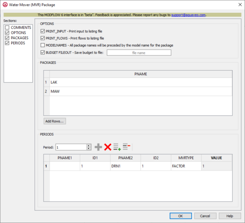
The Water Mover (MVR) Package dialog is accessed by double-clicking on the MVR package under a MODFLOW 6 simulation in the Project Explorer. It contains the following sections and options:
- Sections list – A list of sections that can be turned on or off:
- Comments – Turn on to make the Comments section visible.
- Options – Turn on to make the Options section visible.
- Pacakges – TUrn on to make the Packages section visible.
- Periods – Turn on to make the Periods section visible.
- Comments section – Enter general alphanumeric comments. Comments entered here get written at the top of the file, preceded by a '#' symbol.
- Options section – Temporal options and settings:
- PRINT_INPUT – Print input to listing file. Turn on to write the list of MVR information to the listing file immediately after it is read.
- PRINT_FLOWS – Print flows to listing file. Turn on to write the list of MVR flow rates to the listing file for every stress period time step in which "BUDGET PRINT" is specified in Output Control.
- MODELNAMES – All package names will be preceded by the model name for the package.
- BUDGET_FILEOUT – Save budget to file. Allows the specification of a file to which desired MVR flow terms will be written.
- Packages section – Allows entering the packages which will work with the MVR package.
- Add Rows – Click to bring up the Rows to Add dialog where the number of rows to add to the bottom can be specified.
- Periods section – Contains the following:
- Period drop-down – Use the Increment Up and Down
 buttons to select the desired period.
 - Define Period
 – If no period is defined, click to make the spreadsheet editable.
 - Delete Period
 – Click to delete the existing period.
 - Add Rows
 – Click to bring up the Add Stresses dialog.
 - Delete Rows
 – Click to bring up a dialog with three options:
- Delete from All Periods – Click to delete matching stresses from all periods.
- Delete from Just This Period – Click to delete matching stresses from just this period.
- Plot All Periods
 – Click to bring up the XY Series Editor dialog. Requires that a cell be selected in the table.
 - Open Time Series
 – Click to bring up the
 - Filter on Selected Cells
 – Click to turn on filtering on the selected cells.
 - Table – Options include:
- PNAME1 – The name of a package that may be included in a subsequent stress period block.
- ID1 – Identifies the provider.
- PNAME2 – Represents the package name for the receiver.
- ID2 – The identifier for the receiver.
- MVRTYPE – Is the character that represents the method for determining how much water will be moved.
- VALUE – Is used in an equation to determine how much water will be moved.
- Period drop-down – Use the Increment Up and Down
OBS
| MODFLOW 6 | |
|---|---|
| Models & Tools | |
|
GWF Model GWT Model Cell Properties Dialog Zone File | |
| Packages | |
| Flow: | GNC, HFB, NPF |
| GWF: |
BUY, CHD, CSUB, DRN, EVT, GHB, LAK, MAW, MVR, OBS, RCH,RIV, SFR, STO, UZF, WEL |
| GWT: |
ADV, CNC, DSP FMI, IC, IST, LKT, MDT, MST, MVT, MWT, OBS, SFT, SRC,SSM, UZT |
| Other |
DIS, DISU, DISV, IMS, OC, TDIS, PEST |
The Observations (OBS) Package dialog is accessed by double-clicking on the OBS package under a MODFLOW 6 simulation in the Project Explorer. It contains the following sections and options:
- Sections list – A list of sections that can be turned on or off:
- Comments – Turn on to make the Comments section visible.
- Options – Turn on to make the Options section visible.
- Observations – Turn on to make the Observations section visible.
- Options section contains the following:
- DIGITS – Specify number of significant digits written to output
- PRINT_INPUT – Print input to listing file. Indicates that the list of information will be written to the listing file immediately after it is read.
- Observations section – Allows the entering of specific files into the given text box.
- Add File
 – Click to edit and add a file.
 - Delete File
 – Click to delete the existing file.
 - Observations table: – Enables the entering of observation information when a new file has been added.
- OBSNAME – Name of the observation.
- OBSTYPE – Type of the observation file being used.
- LAY1 – Identifier for the first layer.
- ROW1 – Identifier for the first row.
- COL1 – Identifier for the first column.
- LAY2 – Identifier for the second layer.
- ROW2 – Identifier for the second row.
- COL2 – Identifier for the second column.
- Add Rows... – Allows the inserting of additional rows into the Observations table.
- Add File
OC
| MODFLOW 6 | |
|---|---|
| Models & Tools | |
|
GWF Model GWT Model Cell Properties Dialog Zone File | |
| Packages | |
| Flow: | GNC, HFB, NPF |
| GWF: |
BUY, CHD, CSUB, DRN, EVT, GHB, LAK, MAW, MVR, OBS, RCH,RIV, SFR, STO, UZF, WEL |
| GWT: |
ADV, CNC, DSP FMI, IC, IST, LKT, MDT, MST, MVT, MWT, OBS, SFT, SRC,SSM, UZT |
| Other |
DIS, DISU, DISV, IMS, OC, TDIS, PEST |
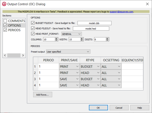
The Output Control (OC) Package dialog is accessed by double-clicking on the OC package under a MODFLOW 6 simulation in the Project Explorer. It contains the following sections and options:
- Sections list – A list of sections that can be turned on or off:
- Comments – Turn on to make the Comments section visible.
- Options – Turn on to make the Options section visible.
- Periods – Turn on to make the Periods section visible. This section is on by default.
- Comments section – Enter general alphanumeric comments. Comments entered here get written at the top of the file, preceded by a '#' symbol.
- Options section contains the following:
- BUDGET_FILEOUT: – Allows the specification of a file to which desired flow terms will be written.
- HEAD_FILEOUT: – Output file to write head information.
- HEAD_PRINT_FORMAT: – When turned on, allows you to specify the format to print to the listing file. Options include:
- "GENERAL" – Prints in the general format to the listing file
- "EXPONENTIAL" – Prints in exponential format to the listing file.
- "FIXED" – Prints in a fixed format to the listing file.
- "SCIENTIFIC" – Prints in a scientific format to the listing file.
- COLUMNS – The number of columns for writing data.
- WIDTH – The width used to write each number
- DIGITS – The number of digits used for writing each number.
- Periods section – Contains the following:
- Add Rows – Click to bring up the Rows to Add dialog where the number of rows to add to the bottom can be specified.
- Preset output – Allows choosing which time periods you wish to output information. Options include:
- "At every time step" – Output information at every time step.
- "At last time step of each stress period" – Output information at the last time step of each stress period.
- "User specified" – Allows user to choose the output settings manually which are entered into a given table.
- Table – Contains the following options:
- PERIOD – Indicates for which PERIOD the information will be saved.
- PRINT/SAVE – Indicates which stress period the information will be printed or saved on.
- RTYPE – This is the type of information (BUDGET/HEAD) to save or print.
- OCSETTING – Indicates which steps the data will be saved for.
- FREQUENCY/STEPS – Indicates which time step frequency or STEPS for which information will be saved.
NPF
| MODFLOW 6 | |
|---|---|
| Models & Tools | |
|
GWF Model GWT Model Cell Properties Dialog Zone File | |
| Packages | |
| Flow: | GNC, HFB, NPF |
| GWF: |
BUY, CHD, CSUB, DRN, EVT, GHB, LAK, MAW, MVR, OBS, RCH,RIV, SFR, STO, UZF, WEL |
| GWT: |
ADV, CNC, DSP FMI, IC, IST, LKT, MDT, MST, MVT, MWT, OBS, SFT, SRC,SSM, UZT |
| Other |
DIS, DISU, DISV, IMS, OC, TDIS, PEST |
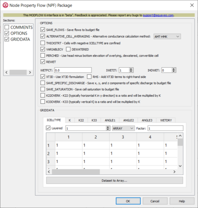
The Node Property Flow (NPF) Package dialog is accessed by double-clicking on the NPF package under a MODFLOW 6 simulation in the Project Explorer. It contains the following sections and options:
- Sections list – A list of sections that can be turned on or off:
- Comments – Turn on to make the Comments section visible.
- Options – Turn on to make the Options section visible.
- GridData – Turn on to make the GridData section visible. This section is on by default.
- Comments section – Enter general alphanumeric comments. Comments entered here get written at the top of the file, preceded by a '#' symbol.
- Options section
- SAVE_FLOWS – Save flows to budget file. Turn on to write cell-by-cell flow terms to the file specified with "BUDGET SAVE FILE" in Output Control.
- ALTERNATIVE_CELL_AVERAGING – Alternative conductance calculation method. Turn on to use an alternative method for calculating the conductance for horizontal cell connections.
- "Logarithmic" –
- "AMT-LMK" – Conductance will be calculated using arithmetic-mean thickness and logarithmic-mean hydraulic conductivity.
- "AMT-HMK" – Conductance will be calculated using arithmetic-mean thickness and harmonic-mean hydraulic conductivity.
- THICKSTRT – Cells with negative ICELLTYPE are confined. Cells having a negative ICELLTYPE are confined, and their cell thickness for conductance calculations will be computed as STRT-BOT rather than TOP-BOT.
- VARIABLECV – Calculate vertical conductance. Vertical conductance will be calculated using the saturated thickness and properties of the overlying cell and the thickness and properties of the underlying cell.
- DEWATERED – Vertical conductance is calculated using only the saturated thickness and properties of the overlying cell if the head in the underlying cell is below its top.
- PERCHED – When a cell is overlying a dewatered convertible cell, the head difference used in Darcy's Law is equal to the head in the overlying cell minus the bottom elevation of the overlying cell.
- REWET – Turn on to activate model rewetting.
- WETFCT – A factor included in the calculation of the head, initially established at a cell when that cell is converted from dry to wet.
- IWETIT – Iteration interval for attempting to wet cells.
- IHDWET – Integer flag that determines which equation is used to define the initial head at cells that become wet.
- XT3D – Use XT3D formulation. Turn on to use the XT3D formulation.
- SAVE_SPECIFIC_DISCHARGE – Turn on to calculate x, y, and z components of specific discharge at cell centers and write them to the cell-by-cell flow file as specified with "BUDGET SAVE FILE" in Output Control.
- SAVE_SATURATION – Save cell saturation to budget file.
- K22OVERK – K22, which is typically the horizontal k in the y-direction, is a ratio and will be multiplied by k.
- K33OVERK – K33, which is typically the vertical k, is a ration and will be multiplied by k.
- GridData section – Contains a number of tabs, including:
- ICELLTYPE – A flag for each cell that specifies how saturated thickness is treated.
- Layered – Turn on if there is more than one affected layer. Select the desired layer from the drop down in order to edit the array (if "Array" is selected from the drop-down).
- If "Constant" is selected from the drop-down, enter a decimal value in the Constant field to be applied to all cells in the layer(s).
- If "Array" is selected from the drop-down, a user-editable array appears below the drop-down. Enter a decimal Factor value to the right of the drop-down. The individual elements of the array are multiplied by the factor value after they are read.
- Dataset to Array... – Click to open the Select Dataset dialog. Select the desired database(s) in this dialog.
- K – The hydraulic conductivity.
- Layered – Turn on if there is more than one affected layer. Select the desired layer from the drop down in order to edit the array (if "Array" is selected from the drop-down).
- If "Constant" is selected from the drop-down, enter a decimal value in the Constant field to be applied to all cells in the layer(s).
- If "Array" is selected from the drop-down, a user-editable array appears below the drop-down. Enter a decimal Factor value to the right of the drop-down. The individual elements of the array are multiplied by the factor value after they are read.
- Dataset to Array... – Click to open the Select Dataset dialog. Select the desired database(s) in this dialog.
- K22 – The hydraulic conductivity of the second ellipsoid axis.
- Define – Turn on if K22 needs to be defined.
- Layered – Turn on if there is more than one affected layer. Select the desired layer from the drop down in order to edit the array (if "Array" is selected from the drop-down).
- If "Constant" is selected from the drop-down, enter a decimal value in the Constant field to be applied to all cells in the layer(s).
- If "Array" is selected from the drop-down, a user-editable array appears below the drop-down. Enter a decimal Factor value to the right of the drop-down. The individual elements of the array are multiplied by the factor value after they are read.
- Dataset to Array... – Click to open the Select Dataset dialog. Select the desired database(s) in this dialog.
- K33 – The hydraulic conductivity of the third ellipsoid axis.
- Define – Turn on if K33 needs to be defined.
- Layered – Turn on if there is more than one affected layer. Select the desired layer from the drop down in order to edit the array (if "Array" is selected from the drop-down).
- If "Constant" is selected from the drop-down, enter a decimal value in the Constant field to be applied to all cells in the layer(s).
- If "Array" is selected from the drop-down, a user-editable array appears below the drop-down. Enter a decimal Factor value to the right of the drop-down. The individual elements of the array are multiplied by the factor value after they are read.
- Dataset to Array... – Click to open the Select Dataset dialog. Select the desired database(s) in this dialog.
- ANGLE1 – The first sequential rotation angle of the hydraulic conductivity tensor in degrees.
- Define – Turn on if ANGLE1 needs to be defined.
- Layered – Turn on if there is more than one affected layer. Select the desired layer from the drop down in order to edit the array (if "Array" is selected from the drop-down).
- If "Constant" is selected from the drop-down, enter a decimal value in the Constant field to be applied to all cells in the layer(s).
- If "Array" is selected from the drop-down, a user-editable array appears below the drop-down. Enter a decimal Factor value to the right of the drop-down. The individual elements of the array are multiplied by the factor value after they are read.
- Dataset to Array... – Click to open the Select Dataset dialog. Select the desired database(s) in this dialog.
- ANGLE2 – The second sequential rotation angle of the hydraulic conductivity tensor in degrees.
- Define – Turn on if ANGLE2 needs to be defined.
- Layered – Turn on if there is more than one affected layer. Select the desired layer from the drop down in order to edit the array (if "Array" is selected from the drop-down).
- If "Constant" is selected from the drop-down, enter a decimal value in the Constant field to be applied to all cells in the layer(s).
- If "Array" is selected from the drop-down, a user-editable array appears below the drop-down. Enter a decimal Factor value to the right of the drop-down. The individual elements of the array are multiplied by the factor value after they are read.
- Dataset to Array... – Click to open the Select Dataset dialog. Select the desired database(s) in this dialog.
- ANGLE3 – The third sequential rotation angle of the hydraulic conductivity tensor in degrees.
- Define – Turn on if ANGLE3 needs to be defined.
- Layered – Turn on if there is more than one affected layer. Select the desired layer from the drop down in order to edit the array (if "Array" is selected from the drop-down).
- If "Constant" is selected from the drop-down, enter a decimal value in the Constant field to be applied to all cells in the layer(s).
- If "Array" is selected from the drop-down, a user-editable array appears below the drop-down. Enter a decimal Factor value to the right of the drop-down. The individual elements of the array are multiplied by the factor value after they are read.
- Dataset to Array... – Click to open the Select Dataset dialog. Select the desired database(s) in this dialog.
- WETDRY – A combination of the wetting threshold and a flag to indicate which neighboring cells can cause a cell to become wet.
- Define – Turn on if WETDRY needs to be defined.
- Layered – Turn on if there is more than one affected layer. Select the desired layer from the drop down in order to edit the array (if "Array" is selected from the drop-down).
- If "Constant" is selected from the drop-down, enter a decimal value in the Constant field to be applied to all cells in the layer(s).
- If "Array" is selected from the drop-down, a user-editable array appears below the drop-down. Enter a decimal Factor value to the right of the drop-down. The individual elements of the array are multiplied by the factor value after they are read.
- Dataset to Array... – Click to open the Select Dataset dialog. Select the desired database(s) in this dialog.
- ICELLTYPE – A flag for each cell that specifies how saturated thickness is treated.
RCH
| MODFLOW 6 | |
|---|---|
| Models & Tools | |
|
GWF Model GWT Model Cell Properties Dialog Zone File | |
| Packages | |
| Flow: | GNC, HFB, NPF |
| GWF: |
BUY, CHD, CSUB, DRN, EVT, GHB, LAK, MAW, MVR, OBS, RCH,RIV, SFR, STO, UZF, WEL |
| GWT: |
ADV, CNC, DSP FMI, IC, IST, LKT, MDT, MST, MVT, MWT, OBS, SFT, SRC,SSM, UZT |
| Other |
DIS, DISU, DISV, IMS, OC, TDIS, PEST |
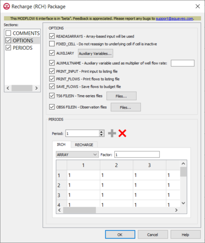
The Recharge (RCH) Package dialog is accessed by double-clicking on the RCH package under a MODFLOW 6 simulation in the Project Explorer. It contains the following sections and options:
- Sections list – A list of sections that can be turned on or off:
- Comments – Turn on to make the Comments section visible.
- Options – Turn on to make the Options section visible.
- Periods – Turn on to make the Periods section visible. This section is on by default.
- Comments section – Enter general alphanumeric comments. Comments entered here get written at the top of the file, preceded by a '#' symbol.
- Options section – Temporal options and settings:
- AUXILIARY – Click the Auxiliary Variables... button to bring up the Auxiliary Variables dialog.
- Time-Array Series Files – Click to bring up the Time-Array Series Files dialog.
- Observations... – Click to bring up the Observation Files dialog.
- Read as arrays (READASARRAYS) – Click to specify to use array-based input in the RCH package.
- Do not reassign to underlying cell if cell is inactive (FIXED_CELL) – Click to indicate that recharge will not be reassigned to a cell underlying the cell specified in the list if the specified cell is inactive.
- Use auxiliary variable as multiplier (AUXMULTNAME) – Name of auxiliary variable to be used as multiplier of recharge.
- Print input to listing file (PRINT_INPUT) – Turn on to write the list of recharge information to the listing file immediately after it is read.
- Print flows to listing file (PRINT_FLOWS) – Turn on to write the list of recharge flow rates to the listing file for every stress period time step in which "BUDGET PRINT" is specified in Output Control.
- Save flows to budget file (SAVE_FLOWS) – Turn on to write recharge flow terms to the file specified with "BUDGET FILEOUT" in Output Control.
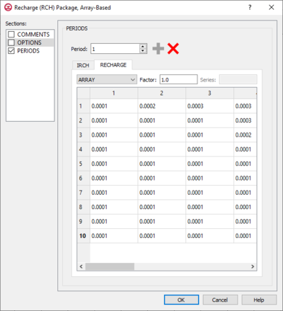
- Periods section – Contains the following:
- Table – Contains two tabs:
- IRCH – The layer number that defines the layer in the column where recharge is applied and can only be applied if READASARRAYS is on in the OPTIONS section.
- "UNDEFINED" – Indicates that there are no definite variables to be applied.
- "CONSTANT" – If "Constant" is selected from the drop-down, enter a decimal value in the Constant field to be applied to all cells in the layer(s).
- "ARRAY" – If "Array" is selected from the drop-down, enter an integer in the factor: field to be multiplied to the array after it is read.
- "TIME_ARRAY SERIES" – Is not supported for IRCH.
- RECHARGE – The recharge flux rate.
- "UNDEFINED" – Indicates that there are no definite variable to be applied.
- "CONSTANT" – If "Constant" is selected from the drop-down, enter a decimal value in the Constant field to be applied to all cells in the layer(s).
- "ARRAY" – If "Array" is selected from the drop-down, enter an integer in the factor: field to be multiplied to the array after it is read.
- "TIME_ARRAY SERIES" – If "Time-Array Series" is selected from the drop-down, indicate which Time-Array Series is being applied in the Series: field.
- IRCH – The layer number that defines the layer in the column where recharge is applied and can only be applied if READASARRAYS is on in the OPTIONS section.
RIV
SFR
STO
UZF
WEL
Simulations Options
New Conceptual Model
New Simulation dialog
New MODFLOW 6 Simulation Dialog
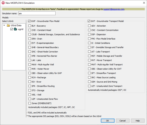
This dialog appears when a new MODFLOW 6 simulation is first created. The dialog has the following options:
- Simulation name – A name for the simulation can be entered in this field.
- Select UGrid – This section will contain a list of available UGrids to use in the MODFLOW 6 simulation. A UGrid must be selected before the simulation can be created.
- Optional packages – This section contains a list of available optional packages that be included when the simulation is created. Packages are listed for both flow and transport model types. The model type must be selected to select the packages associates with the model type. The packages are organized by the model type.
- A message at the bottom of this section will state which packages are already included in the simulation being created.
IMS Package
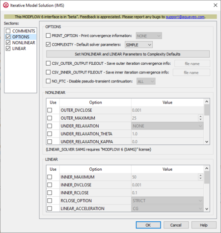
The Iterative Model Solution (IMS) dialog is accessed by double-clicking on the IMS package under a MODFLOW 6 simulation in the Project Explorer. It contains the following sections and options:
- Sections list – A list of sections that can be turned on or off:
- Comments – Turn on to make the Comments section visible.
- Options – Turn on to make the Options section visible.
- Nonlinear – Turn on to make the Nonlinear section visible. This section is on by default.
- Linear – Turn on to make the Linear section visible. This section is on by default.
- Comments section – Enter general alphanumeric comments. Comments entered here get written at the top of the file, preceded by a '#' symbol.
- Options section
- PRINT_OPTION – A flag that controls printing of convergence information from the solver. Turn on to make the following print options available from the drop-down:
- "None" – Print nothing. This is the default when PRINT_OPTION is not turned on.
- "Summary" – Print only the total number of iterations and nonlinear residual reduction summaries
- "All" – Print linear matrix solver convergence information to the solution listing file and model specific linear matrix solver convergence information to each model listing file in addition to "Summary" information.
- COMPLEXITY – Optional. Defines default non-linear and linear solver parameters. Turn on to make the following options available from the drop-down:
- "Simple" – Default solver input values will be defined that work well for nearly linear models.
- "Moderate" – Default solver input values will be defined that work well for moderately nonlinear models.
- "Complex" – Default solver input values will be defined that work well for highly nonlinear models.
- Set NONLINEAR and LINEAR Parameters to Complexity Defaults – This will set all nonlinear and linear parameters to their default values corresponding to the current complexity setting. A confirmation dialog will appear.
- CSV_OUTER_OUTPUT FILEOUT – Turn on to specify that the record corresponds to the comma separated values solver convergence output. Enter the desired filename for the output ASCII CSV file in the empty field to the right of the option.
- CSV_INNER_OUTPUT FILEOUT – Turn on to specify that the record corresponds to the comma separated values solver convergence output. Enter the desired filename for the output ASCII CSV file in the empty field to the right of the option.
- NO_PTC – Turn on to disable pseudo-transient continuation (PTC). Only applies to steady-state stress periods for models using the Newton-Raphson formulation.
- "ALL"
- "FIRST"
- PRINT_OPTION – A flag that controls printing of convergence information from the solver. Turn on to make the following print options available from the drop-down:
- Nonlinear section – A table with three columns: "Use" to turn on or off options, "Option" (giving the name of the option), and "Value", where a value can be entered for the option. The options include the following:
- OUTER_DVCLOSE – Real value defining the head change criterion for convergence of the outer (nonlinear) iterations, in units of length. Default value is "0.001".
- OUTER_MAXIMUM – Integer value defining the maximum number of outer (nonlinear) iterations. Default value is "25".
- UNDER_RELAXATION – Optional drop-down value. Defines the nonlinear under-relaxation schemes used.
- "None" – Under-relaxation is not used.
- "Simple" – Simple under-relaxation scheme with a fixed relaxation factor is used.
- "Cooley" – Cooley under-relaxation scheme is used.
- "DBD" – Delta-bar-delta under-relaxation is used.
- UNDER_RELAXATION_THETA – Real value defining the reduction factor for the learning rate (under-relaxation term) of the delta-bar-delta algorithm. Default value is "0.0".
- UNDER_RELAXATION_KAPPA – Real value defining the increment for the learning rate (under-relaxationterm) of the delta-bar-delta algorithm. Default value is "0.0".
- UNDER_RELAXATION_GAMMA – Real value defining the history or memory term factor of the delta-bar-delta algorithm. Default value is "0.0".
- UNDER_RELAXATION_MOMENTUM – Real value defining the fraction of past history changes that is added as a momentum term to the step change for a nonlinear iteration. Default value is "0.0".
- BACKTRACKING_NUMBER – Integer value defining the maximum number of backtracking iterations allowed for residual reduction computations. Default value is "0".
- BACKTRACKING_TOLERANCE – Only available if BACKTRACKING_NUMBER" has a value of "1" or higher. Real value defining the tolerance for residual change that is allowed for residual reduction computations
- BACKTRACKING_REDUCTION_FACTOR – Only available if BACKTRACKING_NUMBER" has a value of "1" or higher. Real value defining the reduction in step size used for residual reduction computations
- BACKTRACKING_RESIDUAL_LIMIT – Only available if BACKTRACKING_NUMBER" has a value of "1" or higher. Real value defining the limit to which the residual is reduced with backtracking.
- LINEAR_SOLVER – Enter the linear solver being used.
- Linear section – A table with three columns: "Use" to turn on or off options, "Option" (giving the name of the option) and "Value", where a value can be entered for the option. The options include the following:
- INNER_MAXIMUM – Integer value defining the maximum number of inner (linear) iterations. Default value of "50".
- INNER_DVCLOSE (length) – Real value defining the head change criterion for convergence of the inner (linear) iterations, in units of length. Default value of "0.001".
- INNER_RCLOSE (length3/time) – Real value that defines the flow residual tolerance for convergence of the IMS linear solver and specific flow residual criteria used. Default value of "0.1".
- RCLOSE_OPTION – Optional. Defines the specific flow residual criterion used. Default selection of "None". Has the following options:
- "None" – If selected, an absolute residual (infinity-norm) criterion is used.
- "Strict" – Specifies that INNERRCLOSE represents an infinity-Norm (absolute convergence criteria) and that the head and flow convergence criteria must be met on the first inner iteration.
- "L2NORM_RCLOSE" – Specifies that INNERRCLOSE represents a L-2 Norm closure criteria instead of an infinity-Norm (absolute con-vergence criteria).
- "RELATIVE_RCLOSE" – Spcifies that INNERRCLOSE represents a relative L-2 Norm reduction closure criteria instead of an infinity-Norm (absolute convergence criteria).
- LINEAR_ACCELERATION – Defines the linear acceleration method used by the default IMS linear solvers. Default selection of "CG". Has the following options:
- "CG" – Preconditioned conjugate gradient method.
- "BICGSTAB" – Preconditionedbi-conjugate gradient stabilized method.
- RELAXATION_FACTOR – Optional. Real value that defines the relaxation factor used by the incomplete LU factorization preconditioners (MILU(0) and MILUT). Default value of "0.0".
- PRECONDITIONER_LEVELS – Optional. Integer value defining the level of fill for ILU decomposition used in the ILUT and MILUT preconditioners. Default value of "0".
- PRECONDITIONER_DROP_TOLERANCE – Optional. Real value that defines the drop tolerance used to drop preconditioner terms based on the magnitude of matrix entries in the ILUT and MILUT preconditioners. Default value of "0.0".
- NUMBER_ORTHOGONALIZATIONS – Optional. Integer value defining the interval used to explicitly recalculate the residual of the flow equation using the solver coefficient matrix, the latest head estimates, and the right hand side. Default value of "0".
- SCALING_METHOD – Optional. Defines the matrix scaling approach used. Default selection of "None". Has the following options:
- "None" – No matrix scaling applied.
- "Diagonal" – Symmetric matrix scaling using the POLCG preconditioner scaling method.
- "L2NORM" – Symmetric matrix scaling using the L2 norm.
- REORDERING_METHOD – Optional. Defines the matrix reordering approach used. Default selection of "None". Has the following options:
- "None" – Original ordering.
- "RCM" – Reverse Cuthill McKee ordering.
- "MD" – Minimum degree ordering.
MODFLOW 6 Right-Click Menu
In the Project Explorer, right-clicking on MODFLOW 6 simulation brings up a menu with several commands. Some of these commands are common to other Project Explorer right-click menus. Others are unique to the simulation right-click menus. Some of these unique commands are:
- "
 Simulation Data"
- Simulation Run Queue – Opens the Simulation Run Queue dialog which shows all current simulation runs.
- "
 MODFLOW 6 Simulations"
- New Simulation – Creates a new MODFLOW 6 simulation in the Project Explorer. This simulation will not contain any of the packages in any existing simulations and therefor the packages must be added. Also, creating a new simulation using this method requires linking a UGrid to the simulation.
- Simulation Run Queue – Opens the Simulation Run Queue dialog which shows all current simulation runs.
- Save All and Run – Saves all MODFLOW 6 simulations in the project and exports all files needed for the model run. It then will launch the Simulation Run Queu dialog and begin the model runs for all simulations in the project.
 Model
Model
- Simulation Run Queue – Opens the Simulation Run Queue dialog which shows all current simulation runs.
- New Package – Opens a sub-menu listing all available packages that can be added to the simulation. Selecting a package will add it to the simulation. Some packages cannot be added until certain packages have already been added to the simulation and therefore will not be available until the prerequisite package has been added.
- Check Simulation – Checks the simulation for model errors and brings up the Model Check dialog if any errors are found.
- Save Simulation – Saves the simulation and exports all files needed for the model run.
- Run Simulation – Starts the simulation model run and opens the Simulation Run Queue dialog.
- Save Project, Simulation and Run – Saves the simulation and exports all files needed for the model run. It then will launch the Simulation Run Queu dialog and begin the model runs for the simulation.
- Read Solution – Loads the solution file for the associated simulation. Requires that the simulation has had a successful run.
Unsupported Features
In GMS, some features of MODFLOW 6 are not yet supported or only have minimal support. These include:
- MODFLOW 6 features
- Only support for one SOLUTIONGROUP in the mfsim.nam file
- ‘NONE’ for cellid in SFR PACKAGEDATA block is not supported
- IPRN variable for arrays
- Advanced package output files
- GMS interface functionality
- Conceptual model approach for some packages
- Observations coverage
- Cell properties for array-based RCH and EVT packages
The MODFLOW 6 export option does not function with projects that are incompatible with MODFLOW 6. Projects with unsupported features or parameters will not be successfully exported.
Not all MODFLOW packages are supported in MODFLOW 6. The following table shows the correlation between MODFLOW 6 packages and packages from previous versions of MODFLOW.
| MODFLOW 6 supported packages | Equivalent Mf2k5/USG package |
|---|---|
| CHD, DRN, GHB, RIV, WEL | CHD, DRN, GHB, RIV, WEL |
| DIS, DISV, DISU, TDIS | DIS, DISU |
| EVT, RCH | EVT, ETS, RCH |
| GNC | GNC |
| IC | BAS |
| LAK | LAK |
| MAW | MNW2 |
| NPF, STO | BCF, HUF, LPF, UPW |
| SFR | SFR |
| UZF | UZF |
| MVR, GWF, OBS | Not supported |
| Not Supported | DRT, GAGE, MNW1, MNWI, STR, SUB, SWI, OBS, HOB, CHOB, RVOB, STOB, DROB |

