WMS:GSSHA Automated Calibration: Difference between revisions
No edit summary |
|||
| Line 188: | Line 188: | ||
[[Category:GSSHA|C]] | [[Category:GSSHA|C]] | ||
[[Category:GSSHA Dialogs]] | [[Category:GSSHA Dialogs|Cal]] | ||
Revision as of 15:03, 26 August 2016
The GSSHA model allows for both automatic (auto) calibration and manual calibration.
Auto Calibration
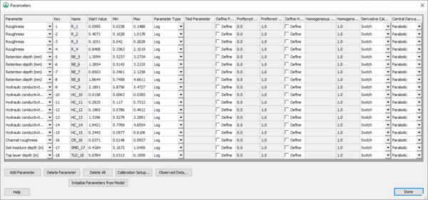
GSSHA has a PEST-based automated calibration routine that is described on the GSSHA wiki. WMS writes the parameters, observed data, and calibration files necessary to run GSSHA in any of the supported GSSHA calibration modes. There is a tutorial included in the WMS Tutorials that describes how to setup a basic calibration model. Enter in the needed data by toggling Calibration in the Job Control dialog. Clicking on the Edit Parameters button allows selection of which parameters are to be calibrated and edit the calibration settings associated with each of the parameters. The dialog shown below appears. Here enter the maximum, minimum, and initial values for each parameter.
Defining Key Values
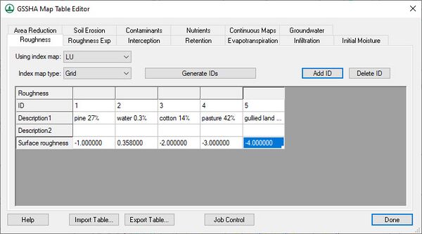
Select adjustable parameters by defining key values as negative numbers in the regular GSSHA interface and then assigning starting, min, and max values to each of these parameters in the calibration interface. For example, if wanting to set overland Manning’s roughness values as an adjustable model parameter, specify negative integers for the values in the mapping table dialog as shown below:
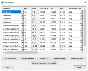
Then define the key values in the calibration Parameters dialog as shown below:
The Initialize Parameters from Model button makes defining key values easy. This button searches the model for any parameters that are defined as negative integers and assigns these parameters to the dialog. For each key value, define a start, min, and max value for the calibration engine. Also define other parameter information, such as whether parameters are fixed or tied to other parameters and the methods used to calculate derivatives for each parameter. Options exist to define regularization parameters that define prior information for the calibration run. There are options to define preferred values, where a specific value is set as an optimal value for the calibration parameter, or homogeneous values, where one or more calibration parameters are linked to another calibration parameter in an attempt to get these values as close as possible.
Defining Observed Data
Clicking the Observed Data... button in the Calibration Parameters dialog opens another dialog, which is shown below. In this dialog, enter in various types of observed data (including time series hydrograph data) for each event of the simulation. It is not necessary to associate a rainfall event with each observed data time series unless running an SCE-type simulation. This dialog shows all the feature points with observed data and allows turning automated calibration on or off for each of these observations. An SCE-type automated calibration simulation can only be used to calibrate the hydrograph at the outlet point and has been deprecated in the current version of WMS. All other automated calibration methods support automated calibration of the following data types at any computation point in the watershed model:
- Overland Depth
- Infiltration Depth
- Surface Moisture
- Grid Suspended Sediment (TSS) Concentration
- Channel Depth
- Channel Flow
- Channel Total Suspended Sediment (TSS) Concentration
- Groundwater Head
- Outlet Hydrograph (Only at the watershed outlet point)
- Snow Water Equivalent
- Tile Drain Discharge (In a GSSHA Storm Drain coverage)
The Observation dialog can be accessed from the feature point/node attribute dialog in the GSSHA and the GSSHA Storm Drain coverages. If WMS is running the default LM/SLM-based calibration, associate weights with each observation value in the XY series by clicking on the Weights button in the observation window and defining weights for each value. WMS defaults all the weights for observed data points to 1.0, but this value could be modified to give higher weights to certain observed values.
Defining Calibration Setup Parameters
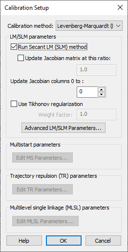
Lastly, set the calibration setup parameters, which can be accessed by clicking the Calibration Setup... button. The following dialog will appear:
The parameters in this dialog are used for the calibration control file. This file, along with the parameters and observed data files are written out by WMS when saving a GSSHA project.
The following options are of note in this dialog:
Calibration method
The following calibration methods are available: Levenberg-Marquardt (LM)/Secant LM (SLM), Multistart (MS), Trajectory Repulsion (TR), Multilevel Single Linkage (MLSL), and Shuffled Complex Evolution (SCE). The LM and SLM methods use a local search to optimize model parameters while the other methods are global search methods. You can find more detailed information about each of these optimization methods on the GSSHA wiki. The SCE method can be considered a deprecated optimization method in GSSHA. Use one of the other optimization methods to optimize your model.
Run Secant LM (SLM) method
Turning on the option to run the SLM method sets the input file flag to run the SLM method instead of the LM (Levenberg-Marquardt) local search method. The SLM method is an efficiency enhancement to the LM method and is the default local search optimization method for a GSSHA calibration in the WMS interface.
Use Tikhonov regularization
Often, when you define preferred values or homogeneous parameter values in a calibration model using the PEST-based prior information (regularization) option, it is desirable to find a balance between fitting the solution to the observed data and fitting to the regularization relationships. The Tikhonov regularization option provides a way to adjust this balance by defining a regularization weight factor and running Tikhonov regularization using this weight factor. This weight factor balances finding a solution that matches observed data versus fitting prior information (regularization) relationships. See the GSSHA wiki for more information about Tikhonov regularization with GSSHA.
Advanced Calibration Parameters
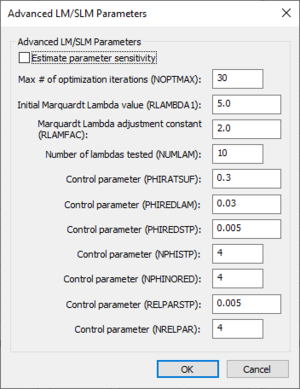
Sometimes, it's desired to set more advanced calibration settings when running an LM/SLM calibration. These settings can be set in the Advanced LM/SLM Parameters dialog and are described below:
Estimate parameter sensitivity
Turn this option on to write a -1 to the NOPTMAX parameter in the PEST control file. This tells PEST to only run a sensitivity analysis instead of a full parameter optimization run. The sensitivity file is read into WMS if reading the calibration solution.
(The descriptions below are taken from the PEST User Manual, Copyright 2013)
NOPTMAX
This sets the maximum number of optimisation iterations that PEST is permitted to undertake on a particular parameter estimation run. If wanting to ensure that PEST termination is triggered by other criteria more indicative of parameter convergence to an optimal set or of the futility of further processing, set this variable very high. A value of 20 to 30 is often appropriate.
If NOPTMAX is set to zero, PEST will not calculate the Jacobian matrix. Instead it will terminate execution after just one model run. This setting can thus be used when wanting to calculate the objective function corresponding to a particular parameter set and/or to inspect observation residuals corresponding to that parameter set.
RLAMBDA1
This real variable is the initial Marquardt lambda. PEST attempts parameter improvement using a number of different Marquardt lambdas during any one optimization iteration; however, in the course of the overall parameter estimation process, the Marquardt lambda generally gets smaller. An initial value of 1.0 to 10.0 is appropriate for most models, though provide a higher initial Marquardt lambda if PEST complains that the normal matrix is not positive definite .
For high values of the Marquardt lambda the parameter estimation process approximates the steepest-descent method of optimization. While the latter method is inefficient and slow if used for the entirety of the optimization process, it often helps in getting the process started, especially if initial parameter estimates are poor.
RLAMFAC
RLAMFAC, a real variable, is the factor by which the Marquardt lambda is adjusted. RLAMFAC must be greater than 1.0. When PEST reduces lambda it divides by RLAMFAC; when it increases lambda it multiplies by RLAMFAC. PEST reduces lambda if it can. However if the normal matrix is not positive definite or if a reduction in lambda does not lower the objective function, PEST has no choice but to increase lambda.
NUMLAM
This integer variable places an upper limit on the number of lambdas that PEST can test during any one optimization iteration. It should normally be set between 5 and 10. For cases where parameters are being adjusted near their upper or lower limits, and for which some parameters are consequently being frozen (thus reducing the dimension of the problem in parameter space) experience has shown that a value closer to 10 may be more appropriate than one closer to 5; this gives PEST a greater chance of adjusting to the reduced problem dimension as parameters are frozen.
PHIRATSUF
During any one optimization iteration, PEST may calculate a parameter upgrade vector using a number of different Marquardt lambdas. First it lowers lambda and, if this is unsuccessful in lowering the objective function, it then raises lambda. If, at any stage, it calculates an objective function which is a fraction PHIRATSUF or less of the starting objective function for that iteration, PEST considers that the goal of the current iteration has been achieved and moves on to the next optimization iteration.
PHIRATSUF (which stands for “phi ratio sufficient”) is a real variable for which a value of 0.3 is often appropriate. If it is set too low, model runs may be wasted in search of an objective function reduction which it is not possible to achieve, given the linear approximation upon which the optimization equations are based. If it is set too high, PEST may not be given the opportunity of refining lambda in order that its value continues to be optimal as the parameter estimation process progresses.
PHIREDLAM
If a new/old objective function ratio of PHIRATSUF or less is not achieved as the effectiveness of different Marquardt lambdas in lowering the objective function are tested PEST must use some other criterion in deciding when it should move on to the next optimization iteration. This criterion is partly provided by the real variable PHIREDLAM. The first lambda that PEST employs in calculating the parameter upgrade vector during any one optimization iteration is the lambda inherited from the previous iteration, possibly reduced by a factor of RLAMFAC (unless it is the first iteration, in which case RLAMBDA1 is used). Unless, through the use of this lambda, the objective function is reduced to less than PHIRATSUF of its value at the beginning of the iteration, PEST then tries another lambda, less by a factor of RLAMFAC than the first. If the objective function is lower than for the first lambda (and still above PHIRATSUF of the starting objective function), PEST reduces lambda yet again; otherwise it increases lambda to a value greater by a factor of RLAMFAC than the first lambda for the iteration. If, in its attempts to find a more effective lambda by lowering and/or raising lambda in this fashion, the objective function begins to rise, PEST accepts the lambda and the corresponding parameter set giving rise to the lowest objective function for that iteration, and moves on to the next iteration. Alternatively if the relative reduction in the objective function between the use of two consecutive lambdas is less than PHIREDLAM, PEST takes this as an indication that it is probably more efficient to begin the next optimization iteration than to continue testing the effect of new Marquardt lambdas.
A suitable value for PHIREDLAM is often around 0.01. If it is set too large, the criterion for moving on to the next optimisation iteration is too easily met and PEST is not given the opportunity of adjusting lambda to its optimal value for that particular stage of the parameter estimation process. On the other hand if PHIREDLAM is set too low, PEST will test too many Marquardt lambdas on each optimization iteration when it would be better off starting on a new iteration.
PHIREDSTP, NPHISTP
PHIREDSTP is a real variable whereas NPHISTP is an integer variable that are used to tell PEST that the optimization process is at an end. For many cases 0.01 and 4 are suitable values for PHIREDSTP and NPHISTP respectively. However, be careful not to set NPHISTP too low if the optimal values for some parameters are near or at their upper or lower bounds. In this case it is possible that the magnitude of the parameter upgrade vector may be curtailed over one or a number of optimization iterations to ensure that no parameter value overshoots its bound. The result may be smaller reductions in the objective function than would otherwise occur. It would be a shame if these reduced reductions were mistaken for the onset of parameter convergence to the optimal set.
NPHINORED
If PEST has failed to lower the objective function over NPHINORED successive iterations, it will terminate execution. NPHINORED is an integer variable; a value of 3 or 4 is often suitable.
RELPARSTP, NRELPAR
If the magnitude of the maximum relative parameter change between optimization iterations is less than RELPARSTP over NRELPAR successive iterations, PEST will cease execution. PEST evaluates this change for all adjustable parameters at the end of each optimisation iteration, and determines the relative parameter change with the highest magnitude. If this maximum relative change is less than RELPARSTP, a counter is advanced by one; if it is greater than RELPARSTP, the counter is zeroed.
All adjustable parameters, whether they are relative-limited or factor-limited, are involved in the calculation of the maximum relative parameter change. RELPARSTP is a real variable for which a value of 0.01 is often suitable. NRELPAR is an integer variable; a value of 2 or 3 is normally satisfactory.
Calibration Model-Specific Parameters
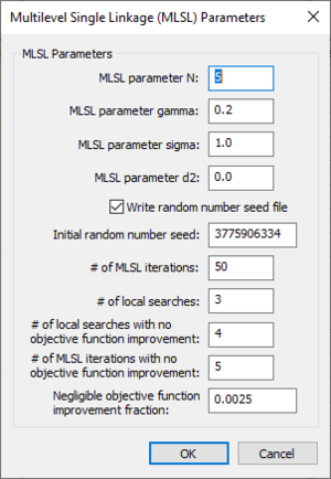
Each calibration model has model-specific calibration parameters. The LM/SLM parameters are local calibration methods and are used with any of the PEST-based global calibration methods as well. The Multistart, TR, and MLSL parameters can be edited by selecting the desired calibration type and then setting the parameters for the calibration in the calibration model dialog, like the MLSL dialog shown below:
Manual Calibration
Manual calibration is the process of changing simulation input so that the simulation output matches observed values. Manual calibration takes a lot of experience and a lot of patience, but it is possible to achieve a good fit between the simulation and the observed data. Being able to successfully manually calibrate a simulation is a necessary skill to successfully set up and run an automatic calibration program.
Steps in the Manual Calibration Process
- Set up and run a successful simulation.
- Identify the calibration variables.
- Decide on a valid range for each variable.
- Set initial values of variables and run the model.
- Compare model results to observed values.
- Change variable values and re-run.
- Repeat steps 5 and 6 until the simulation results closely approximate the observed values.
1. Set up and run a successful simulation
The first step to calibrating a simulation is to set up and successfully run a reasonable simulation. All known parameters, such as precipitation, should be defined; all unknown parameters should be set to physically realistic values. For example, if actual roughness values are unknown then set all of the roughness values to 0.035 or some other reasonable number. Setting the roughness values to 0.00 or some default value will not allow the simulation to proceed. One important consideration is that if the spatial or temporal resolution is too coarse than the simulation will be unduly influenced by numerical issues related to the implementation of the partial differential equations. The result of too coarse of a temporal or spatial resolution will be delayed flows. For more information, see the Primer: Using Watershed Modeling System (WMS) for Gridded Surface Subsurface Hydrologic Analysis (GSSHA) Data Development – WMS 6.1 and GSSHA 1.43c (Downer et. al 2003).
2. Identify the calibration variables
The calibration variables are the simulation parameters whose exact quantities are unknown. This may range from a small handful to several dozen. At this stage it is also often necessary to identify which parameters the simulation is sensitive to and which can be left at good approximations without unduly affecting the model. The number of calibration variables must be pared down to a manageable number as well. Attempting to manually calibrate a simulation with dozens of unknown parameters will lead to one major headache and not to a good, robust simulation. Calibration cannot overcome a general lack of data.
Occasionally lab tests for such parameters as hydraulic conductivity will be available. Such data is very valuable but it still may be necessary to calibrate on that specific parameter because a simulation parameter represents a uniform parameter over an area while lab results generate the parameter for a specific point. The lab data is a very good starting value but may need some modification before it is applicable to a general area.
3. Decide on a valid range for each variable
Knowing a range for each variable is very important. To accurately simulate what is actually present in the watershed requires knowledge of the physical meaning of all of the numerical parameters for the watershed. Without this understanding a simulation that does not accurately reflect reality will be created and the simulation will be worthless in a predictive capacity. Consulting published works that describe the formulas used in GSSHA and detail the values and physical meaning of the formula parameters is highly recommended.
4. Set initial values of variables and run the model
Once the calibration variables have been decided upon and the valid range for each has been identified, the next step is to set an initial value for each variable. The usual process is to begin with the middle value. Later on these values will be modified little by little, either up or down. Beginning with the middle value of the range gives a good reference point for later simulations where what happens with a higher or lower value can be judged against the middle value to determine simulation trends.
5. Compare model results to observed values
This is the key step to calibrating a simulation. Click on the button in the Solution Results column of the Feature Point/Node Properties dialog to display the Solution Analysis dialog, which allows both visual inspection of the solution result as well as numerical evaluation of the “fitness” of a solution. Using these criteria judge how well the simulation output fits the observed.
6. Change variables and re-run
If the simulation output is not sufficiently close to the observed data then the next step is to adjust one or more of the model parameters to try to get a better fit. This step takes practice, experience, and patience. If by adjusting the variables outside of the predefined range a better fit is obtained then either the simulation is poorly set up or the data on which the model is based may be in question. It may also be that the interdependence of variables is such that the other variables in the model should be adjusted before the one that seems to call into question the parameter bounds. After adjusting the variables and running the simulation, check the new output and judge the results of the new variable setting.
Simulation non-uniqueness
One important facet of calibrating a simulation is that often changing more than one variable can have very similar results on the simulation output. Calibrating a simulation attempts to extract spatial simulation parameters from observed data through a process called inverse modeling. Problems arise in calibrating when modifying more than one variable produces only one type of result in the simulation. The question then arises as to which variable values should be the actual variable values. This problem is not solvable and the simulation is said to be non-unique or over-specified. The only way to overcome this problem is by utilizing more data that is of a different type than that already being used. For example, using a stream-flow hydrograph as well as a set of observed groundwater elevations would help eliminate simulation non-uniqueness.
Related Topic
GSSHA | |
|---|---|
| XMS Wiki Links | Calibration (Automated • Manual • Output) • Channel Routing • Contaminants • Digital Dams • Embankment Arcs • Feature Objects (Arcs • Nodes • Polygons) • File Types • Groundwater • Groups • Hydraulic Structures • Job Control • Join SSURGO Data • Mapping Tables • Maps • Menu • Model Linkage • Multiple Simulations • Nutrients • Observations • Output Control • Overland Soil Erosion • Pipe and Node Parameters • Precipitation • Radar Rainfall • Save GSSHA Project File • Smooth GSSHA Streams • Snowmelt • Solution (Analysis • Data) |
| Related Tools | MWBM Wizard • Using Soil Type Data with GSSHA |
| GSSHA Wiki External Links | GSSHA Wiki: Overview • Primer • User's Manual • Tutorials |
