| MODFLOW |
|---|
| Pre-processing |
|---|
|
MODFLOW Commands |
|
Building a MODFLOW Model |
|
Map to MODFLOW |
|
Calibration |
|
Packages Supported in GMS |
|
Saving a MODFLOW Simulation |
|
Importing MODFLOW Files |
|
Unsupported MODFLOW Features |
|
Run MODFLOW |
| Post-processing |
|---|
|
MODFLOW Display Options |
|
MODFLOW Post-Processing Viewing Options |
|
Reading a MODFLOW Simulation |
| Tutorials |
|---|
| Packages |
|---|
| Flow: |
BCF6, HUF, LPF, UPW |
|---|
| Solvers: |
DE4, GMG, NWT, PCG,
PCGN, LMG, SIP, SOR,
SMS |
|---|
| Other: |
BAS6, BFH, CHD1, CLN,
DRN1, DRT1, EVT1, ETS1,
GAGE, GHB1, GNC, HFB1,
HUF, LAK3, MNW1, MNW2,
OUT1, RCH1, RIV1, SFR2,
STR1, SUB1, SWI2, WEL1,
UZF1 |
|---|
|
The MODFLOW SWI2 (SeaWater Intrusion) package is an optional package in MODFLOW-2005 and MODFLOW-NWT. It can be used to model 3D "vertically integrated variable-density
groundwater flow and seawater intrusion in coastal multiaquifer systems."[1]
GMS provides an interface to the SWI2 package. The package can be turned on in the MODFLOW Packages dialog, accessible from the MODFLOW Global/Basic Package dialog. The package dialog can be accessed from the main MODFLOW menu or by right-clicking on the MODFLOW item in the Project Explorer.

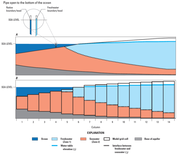
A, cross section through a coastal aquifer with freshwater flowing from right to left and discharging seaward of the coastline;
B, cross section through a coastal aquifer discretized using a single model layer. The position of the freshwater-seawater interface is also shown on
A and
B.
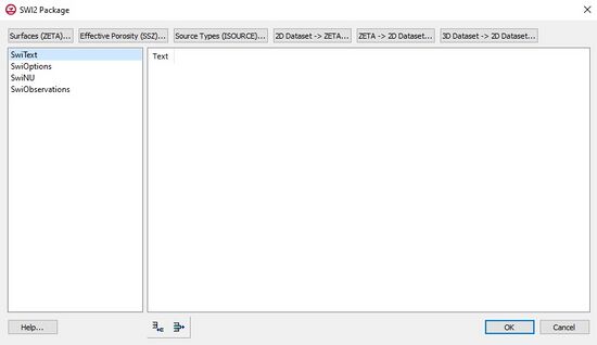
[1] SWI2 Package Dialog
The SWI2 Package dialog allows entering the data needed by the SWI2 package. The dialog includes four tables and some arrays. The tables are as follows:
- SwiText – A list of lines of text (comments) that can appear at the top of the SWI2 package file.
- SwiOptions – A number of variables that control the SWI2 package, consisting of data sets 1-4 in the SWI2 input file. Refer to the SWI2 documentation for the meaning of each variable.
- SwiNU – A list of the dimensionless densities for each zone, or for each surface depending on whether a stratified (ISTRAT = 1) or continuous (ISTRAT = 0) simulation is being used, respectively.
- SwiObservations – A list of observations.
In addition to these four tables, there are three arrays: Surfaces (ZETA), Effective Porosity (SSZ), and Source Types (ISOURCE). These can be accessed via the three buttons on the top left of the dialog.
Zeta Surfaces Input
The Surfaces (ZETA) button opens an array editor dialog which lets the user enter the data for the zeta surfaces. The zeta surfaces are the interfaces between zones of water of different densities. For example, one zeta surface may be used two divide freshwater from seawater, or two zones may be used to divide freshwater from brackish water and brackish water from seawater. All surfaces are specified in each model layer. This can be confusing. Although we typically think of the freshwater-seawater interface as a two-dimensional surface, the SWI2 package requires the surface be specified for every layer, which makes it a 3D array. As explained in the documentation:
"An elevation for each surface needs to be specified for every cell in the model... For the case of a surface that is present at only one point in the vertical everywhere, the same grid of zeta values may be entered for every model layer and SWI2 will determine in which cells the elevation of the zeta surface falls between the top and [bottom] of each layer..."[1]
The zeta surfaces must be reasonably smooth or they may create difficulties for MODFLOW and MODFLOW may have a harder time converging.
There are a number of options for entering the zeta surface data, including:
- Entering the data by hand in the array editor dialog, or copy/pasting from a spreadsheet for each layer.
- Copying a 2D dataset to each layer of the zeta surface array via the 2D Dataset → ZETA button in the SWI2 Package dialog. This requires a 2D grid which matches the 3D grid. A dataset on the 2D grid is chosen and intelligently copied to the zeta arrays.
- Copying a 3D dataset on the 3D grid to the zeta surface array using the 3D Dataset → Grid button in the array editor dialog. The 3D dataset may be created by interpolating from 2D scatter points or a raster.
Post-processing
The SWI2 package output can include a file that contains the calculated positions of the zeta surfaces for every time step. The file is format is that of a budget file—the same as the CCF file. To visualize the calculated surfaces, the surface data must first be converted to 3D datasets by right-clicking on the budget file and selecting the CCF → Datasets command. These datasets can be contoured on the grid, but a more natural way of viewing the data is to create a 2D surface by using the 3D Dataset → 2D Dataset button in the SWI2 Package dialog. This button launches an algorithm which intelligently converts the 3D dataset to a 2D surface. A 2D grid which matches the 3D grid in X and Y is required. The resulting 2D dataset can be animated over time.
Unfortunately at this time GMS is not able to animate more than one surface at a time because there can only be one 2D grid at a time. Also, although multiple TINs can exist at the same time, only the active TIN will be animated. This is a shortcoming that will be addressed in a future version of GMS.
Notes
- ^ a b c
Bakker, Mark, Schaars, Frans, Hughes, J.D., Langevin, C.D., and Dausman, A.M., (2013), Documentation of the Seawater Intrusion (SWI2) Package for MODFLOW: U.S. Geological Survey Techniques and Methods, book 6, chap. A46, 47 p.,, http://pubs.usgs.gov/tm/6a46/

