Lidar: Difference between revisions
No edit summary |
|||
| Line 26: | Line 26: | ||
:Lidar points may be excluded by XYZ extents as well as by either classification or lidar return type. | :Lidar points may be excluded by XYZ extents as well as by either classification or lidar return type. | ||
[[File:LidarExclusionExtents.png|thumb| | [[File:LidarExclusionExtents.png|thumb|330 px|The ''Lidar Exclusion Extents'' dialog]] | ||
''Exclusion extents'' | ''Exclusion extents'' | ||
:If the ''Exclusion extents'' option is turned on, an '''Options''' button is enabled that, when clicked, opens the ''Lidar Exclusion Extents'' dialog. This dialog allows for a minimum and maximum XYZ range to be specified. All points outside this range will be excluded. The XY range, or the Z range, or both can be used to exclude points. If the XY range is being used to exclude points, and if the display is currently in [[GMS:Display Menu|plan view]], an option is available to update the minimum and maximum XY range using the current view. Selecting the '''Update''' button causes the bounds of the current view to be copied to the table. | :If the ''Exclusion extents'' option is turned on, an '''Options''' button is enabled that, when clicked, opens the ''Lidar Exclusion Extents'' dialog. This dialog allows for a minimum and maximum XYZ range to be specified. All points outside this range will be excluded. The XY range, or the Z range, or both can be used to exclude points. If the XY range is being used to exclude points, and if the display is currently in [[GMS:Display Menu|plan view]], an option is available to update the minimum and maximum XY range using the current view. Selecting the '''Update''' button causes the bounds of the current view to be copied to the table. | ||
Revision as of 23:01, 29 November 2022
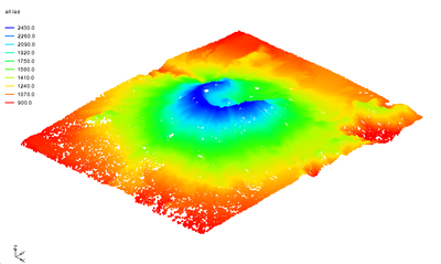
Lidar data is surveying data created by taking measurements with pulsed laser light. Lidar data can be used in XMS software for display and interpolation. Lidar is typically used to get elevation data for use in a model.
Lidar files typically have a *.las or *.laz extension. The *.laz extension is simply a compressed *.las file. XMS software can read both types of files. When a lidar file is opened it appears in the Project Explorer with this icon ![]() under GIS Layers.
under GIS Layers.
Lidar Display Options
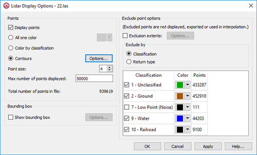
The Lidar Display Options dialog can be accessed by right-clicking on the lidar object in the Project Explorer. Note that currently this is the only way to access the Lidar Display Options dialog and that the main Display Options dialog does not include lidar options. Each lidar object has its own display options which can be set independently of other lidar files’ display options.
The left side of the dialog shows options for displaying points and a bounding box, and the right side shows options for excluding points.
Point Color
- Lidar points can be colored all the same color, or according to their classification, or by using contour options. The lidar contour options are the same as contour options used elsewhere in XMS, except that the only Color Method available is "Color Fill".
Max number of points displayed
- Because lidar data is typically quite large, in order to speed up the display of lidar points, the maximum number of lidar points displayed can be set to something less than the total number of points in the file. Points will be sampled based on the order that they appear in the file and the exclusion options.
Bounding box
- A bounding box can be displayed showing the XYZ extents of the data.
Exclude point options
- The right side of the Lidar Display Options dialog shows options used to exclude points. Excluding points is often helpful due to the sheer quantity of lidar data. Excluded points are not displayed, exported, or used when interpolating.
- Lidar points may be excluded by XYZ extents as well as by either classification or lidar return type.
Exclusion extents
- If the Exclusion extents option is turned on, an Options button is enabled that, when clicked, opens the Lidar Exclusion Extents dialog. This dialog allows for a minimum and maximum XYZ range to be specified. All points outside this range will be excluded. The XY range, or the Z range, or both can be used to exclude points. If the XY range is being used to exclude points, and if the display is currently in plan view, an option is available to update the minimum and maximum XY range using the current view. Selecting the Update button causes the bounds of the current view to be copied to the table.
Classifications and Return types
- Lidar files typically include data on point classifications and return types. This data can be used to exclude points.
- Exclude by classification
- If the Classification option is selected in the Exclude by section, a table shows all the classifications found in the file. Only checked classifications will be included. If Color by classification is chosen (under Points on the left of the dialog), a color can be specified for each classification and those colors will be used in the display. The Points column in the table gives the total number of points for each classification. By default, low point noise is excluded when opening a lidar file.
- Exclude by return type
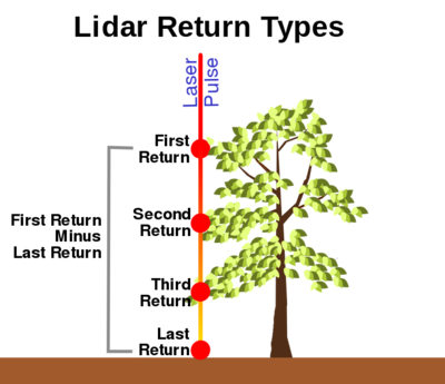
- If the Return type option is selected, the table shows four possible return types. The following figure illustrates what is meant by a lidar “return”.
- Each lidar point includes two numbers related to the laser pulse: the total number of returns, and the points’ return number. A return type is a combination of these two numbers. XMS currently lists four return types that may be useful when excluding points:
- If the Return type option is selected, the table shows four possible return types. The following figure illustrates what is meant by a lidar “return”.
- Single and Last-of-many – This is actually two return types, both of which imply the last point, which is typically the ground surface.
- First-of-many – Typically some feature above the ground, such as a tree top, or even a bird.
- Second but not-last – Typically lower vegetation. Not the ground.
- First – Could be anything, as it may also be the last point.
- A point may be included in more than one return type, for example, a first point would be included in 2, first-of-many, and 4, first.
Lidar Conversion for use in Interpolation
SMS includes functionality to convert lidar data to UGrids (see GMS UGrid and SMS UGrid) and Rasters (see GMS Rasters and SMS Rasters). These options find their applicability in the fact that lidar cannot be used directly as a source of interpolation. The commands to interpolate a lidar file are found in the right-click menu.
- Interpolate to UGrids
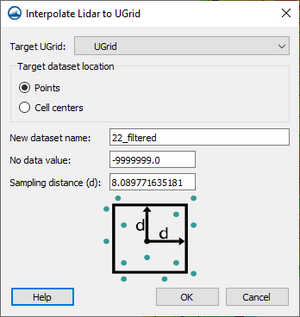
- One or more lidar files can be interpolated to a UGrid points or cell centers to create a new dataset. The lidar points lying within a square defined by a sampling distance are averaged to provide a data value that is then assigned to the UGrid point or cell.
- If there are sparse areas in the lidar that would potentially leave “holes” in the dataset, SMS and GMS will attempt to fill these holes by interpolating from the surrounding cells. If the hole is not completely surrounded by cells with valid interpolated values, cells in the hole will be assigned the No data value.
- Note: Currently WMS does not support this feature.
- Interpolate (conversion) to Raster
- Lidar data can be used to create a new raster. Unlike lidar, rasters are uniformly gridded data. This structured nature makes rasters more efficient to store and work with.
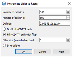
- When converting a lidar data set to raster format, XMS fits the raster to bound the active point in the lidar set. The user specifies the cell size or resolution (number of cells) used to fill this area. Each active point in the lidar is then mapped to the cell containing that point. If more than one active point maps to a single cell, the lidar values are averaged to determine the raster cell value. Any cells not containing at least one lidar point are identified as NODATA cells.
- The Aquaveo software has 3 options to determine data values for raster cells that do not contain any lidar points (these are referred to as NODATA cells). The 3 options are:
- Don't fill NODATA cells: This option leaves NODATA cells as voids (holes) in the raster. This option may be utilized to identify unclassified regions in a lidar set such as buildings or water surface. This option should be used when such voids are desired.
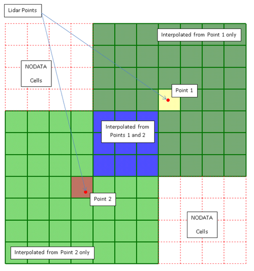
- Fill NODATA cells with filter: (Default option) This option spreads data values from raster cells containing at least one active lidar point to neighboring NODATA cells to minimize the existence of holes. This results in less possibility of missing values when using the raster as the source of interpolation. This option uses a Filter size (in each direction) to determine how far a filled raster cell can spread. This value is specified in the Interpolate Lidar to Raster dialog. This filter size specifies the number of cells in each direction from the cell with the active LIDAR point to interpolate a value based on the following inverse distance weight equation:
- Wi = 1.0 / (1.0 + Fd (Dx2 + Dy2))
- Where:
- Wi = The weight of the lidar point at the current raster cell,
- Fd = The distance factor, currently equal to 1.0 x 10⁶,
- Dx2 = The X distance from the current raster cell to the raster cell with the lidar point, in number of pixels, and
- Dy2 = The Y distance from the current raster cell to the raster cell with the lidar point, in number of pixels.
- The values for any raster cells influenced by more than one lidar point within the specified filter size are interpolated and weighted according to the equation described above. The large value for the distance factor strongly favors values lying in the raster cell since the distance factor term would be set to zero for these cells. Any NODATA cells within filter pixels of cells with data will be assigned a value, thus reducing the size of the hole in the raster.
- Interpolate (beta): This option interpolates from active cells using linear interpolation. After determining the cells containing at least one active LIDAR point and averaging the LIDAR values for these cells, the entire raster is divided into 1000 X 1000 cell tiles, the active points in each of these sections is triangulated, and values for cells inside the triangulated area with NODATA values are computed using linear interpolation. The 1000 x 1000 tiles start at the lower left corner of the raster. It should be noted that blocks of NODATA cells that lie on the edges or corners of these tiles result in remaining voids in the raster. This method is in beta mode and should be used with caution.
Merging Lidar Files
Multiple files can be merged into one file. This is done by selecting the lidar files in the Project Explorer, right-clicking, and selecting the Merge command. All the lidar files to be merged must have the same projection.
Since each lidar file has its own display options, merging multiple lidar files into one can make it simpler to change the display options for all of the data.
Lidar Commands
Lidar commands are found by right-clicking on a lidar file in the Project Explorer. The menu contains many of the standard commands. Unique commands to lidar files includes:
- Display Options
- Opens the Lidar Display Options dialog where options for displaying lidar data can be set. This is the only way to reach this dialog at this time.
- Interpolate to Raster
- Opens the Interpolate Lidar to Raster dialog to create a new raster file.
- Interpolate to UGrid
- Opens the Interpolate Lidar to UGrid dialog to creates a new dataset under a UGrid using the lidar values.
- Convert to 2D Scatter
- Creates a 2D scatter set from the lidar elevation data.
- Merge
- Combines multiple selected lidar files into one lidar file.
- Properties
- Brings up a Properties dialog which displays information about the lidar file.
Related Topics
GMS – Groundwater Modeling System | ||
|---|---|---|
| Modules: | 2D Grid • 2D Mesh • 2D Scatter Point • 3D Grid • 3D Mesh • 3D Scatter Point • Boreholes • GIS • Map • Solid • TINs • UGrids | |
| Models: | FEFLOW • FEMWATER • HydroGeoSphere • MODAEM • MODFLOW • MODPATH • mod-PATH3DU • MT3DMS • MT3D-USGS • PEST • PHT3D • RT3D • SEAM3D • SEAWAT • SEEP2D • T-PROGS • ZONEBUDGET | |
| Aquaveo | ||
SMS – Surface-water Modeling System | ||
|---|---|---|
| Modules: | 1D Grid • Cartesian Grid • Curvilinear Grid • GIS • Map • Mesh • Particle • Quadtree • Raster • Scatter • UGrid |  |
| General Models: | 3D Structure • FVCOM • Generic • PTM | |
| Coastal Models: | ADCIRC • BOUSS-2D • CGWAVE • CMS-Flow • CMS-Wave • GenCade • STWAVE • WAM | |
| Riverine/Estuarine Models: | AdH • HEC-RAS • HYDRO AS-2D • RMA2 • RMA4 • SRH-2D • TUFLOW • TUFLOW FV | |
| Aquaveo • SMS Tutorials • SMS Workflows | ||
WMS – Watershed Modeling System | ||
|---|---|---|
| Modules: | Terrain Data • Drainage • Map • Hydrologic Modeling • River • GIS • 2D Grid • 2D Scatter |  |
| Models: | CE-QUAL-W2 • GSSHA • HEC-1 • HEC-HMS • HEC-RAS • HSPF • MODRAT • NSS • OC Hydrograph • OC Rational • Rational • River Tools • Storm Drain • SMPDBK • SWMM • TR-20 • TR-55 | |
| Toolbars: | Modules • Macros • Units • Digitize • Static Tools • Dynamic Tools • Drawing • Get Data Tools | |
| Aquaveo | ||
