GMS:Global Options/Basic Package: Difference between revisions
No edit summary |
|||
| Line 49: | Line 49: | ||
=== Model Type === | === Model Type === | ||
The simulation can be designated as either | The simulation can be designated as either ''Steady state'' or ''Transient''. If a steady state simulation is specified, certain portions of the MODFLOW interface such as the ''Stress Period'' dialog are inactivated since they are not relevant. | ||
=== No Flow Head === | === No Flow Head === | ||
Revision as of 16:23, 6 February 2017
| MODFLOW | |
|---|---|
| Pre-processing | |
| MODFLOW Commands | |
| Building a MODFLOW Model | |
| Map to MODFLOW | |
| Calibration | |
| Packages Supported in GMS | |
| Saving a MODFLOW Simulation | |
| Importing MODFLOW Files | |
| Unsupported MODFLOW Features | |
| Run MODFLOW | |
| Post-processing | |
| MODFLOW Display Options | |
| MODFLOW Post-Processing Viewing Options | |
| Reading a MODFLOW Simulation | |
| Tutorials | |
| Packages | |
| Flow: | BCF6, HUF, LPF, UPW |
| Solvers: | SMS |
| Other: | UZF1 |
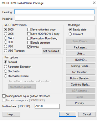
Once the MODFLOW simulation has been initialized, the next step is to enter the data required by the Global Options/Basic package. This includes data defining fundamental program options such as the computational time intervals (stress periods), an array defining which cells are inactive and which cells have constant heads, an array of starting head values for a transient simulation, and a set of flags defining which of the other packages are to be used. The input data for this package should be entered before editing any of the other packages. The MODFLOW Global Options/Basic Package dialog is accessed through the Global Options command in the MODFLOW menu.
The options in the dialog are as follows:
Contents
Headings
The two headings are optional text strings which are written to the MODFLOW text output file.
Version
The MODFLOW version can be specified with the choices being (as of Apr 2014):
- MODFLOW-2000
- MODFLOW-2005
- MODFLOW-NWT
- MODFLOW-LGR
- MODFLOW-USG
The type of binary executable can be specified using one or more of the following choices:
- Double precision – Uses 8 bytes rather than 4 bytes to store the number so they are more precise but calculations may take longer and binary files that store double-precision variables will be bigger than if single-precision had bee used.
- Parallel – Enables parallel processing capabilities.
- 64 bit – Process using 64 bytes to store the number.
The Save native text copy option will save native ascii MODFLOW input files when the project is saved. An additional folder named myProject_MODFLOW_text is created that contains these files.
The Use custom Run dialog option will bring up the Custom Run MODFLOW dialog when the MODFLOW | Run MODFLOW menu command is selected.
The Set as Default button will set the selected model run options as the default MODFLOW model run options for GMS.
Run Options
The run options are not part of the actual MODFLOW input files, but present different ways that MODFLOW 2000 can be run from GMS.
Forward Run
- A Forward run is a normal MODFLOW simulation. If parameters have been defined for either a stochastic or parameter estimation run, the mean or starting values of the parameters are used for the forward run.
Sensitivity Analysis
- The Sensitivity Analysis option is used to perform a sensitivity analysis on a set of selected parameters. The results can be presented with a set of plots or by contouring datasets representing grid sensitivities. This option is only available with the LPF and HUF flow packages. This option is not available in GMS 6.5 and later (see MODFLOW with HDF5).
- After running PEST, sensitivities are displayed in the *.sen file. Click here for more information.
Parameter Estimation
- In the Parameter Estimation mode, a set of parameters is found that minimizes the residual between observed and simulated heads and flows. These options are described in more detail on the Automated Parameter Estimation page. This option is only available with the LPF and HUF flow packages.
Stochastic Simulation
- The Stochastic Simulation option is used to perform a stochastic simulation using the Monte Carlo or Latin Hypercube methods for randomizing a selected set of parameters. Stochastic simulations can also be performed using a material set approach (indicator simulations). A risk analysis wizard can be used to analyze the results for a probabilistic threshold analysis or a probabilistic capture zone delineation. These options are described in more detail on the stochastic simulation page.
Stochastic Inverse Model
- If the Material Set option is used for stochastic simulations, the Stochastic Inverse option can be used to perform automated parameter estimation on each of the N candidate model instances in the stochastic. The weighted RMS errors for each of the resulting optimized solutions can be used to weight the computations performed by the risk analysis wizard. This option is only available with the LPF and HUF flow packages.
Model Type
The simulation can be designated as either Steady state or Transient. If a steady state simulation is specified, certain portions of the MODFLOW interface such as the Stress Period dialog are inactivated since they are not relevant.
No Flow Head
This is the value of head to be assigned to all inactive (no flow) cells (IBOUND=0) throughout the simulation.
Stress Periods
The Stress Periods button is used to bring up the Stress Period dialog. The stress periods should be defined before any of the sources/sinks are entered. If the steady state option is selected, the Stress Periods button is dimmed.
Packages
The Packages button brings up the Packages dialog.
Units
The Units button the Basic Package dialog brings up the Units dialog.
IBOUND
Values
The IBOUND button of the Global Options\Basic Package dialog brings up the Array Editor. The IBOUND array contains a value for each cell in the grid defining the type of the cell as constant head, inactive, or variable head.
Constant Head
- A negative value indicates that the cell has a constant head. The value of the constant head is defined in the starting heads array.
Inactive
- An IBOUND value of zero indicates that the cell is inactive (no-flow).
Variable Head
- A positive IBOUND value indicates that the cell has a variable head (i.e., the head value will be computed as part of the simulation).
Editing the IBOUND Array
There are several ways to change the active/inactive status (positive vs. zero) of a cell before or after initializing the IBOUND array. One method is to directly edit the IBOUND array using the IBOUND dialog. Another method is to select the Cell Attributes command in the MODFLOW menu. In most cases, the most efficient method is to use the Activate Cells in Coverage command in the Map module. This method uses a polygon to define the active and inactive regions.
The constant head cells are typically assigned or edited in one of three ways. One method is to directly edit the IBOUND array. Another method is to select a set of cells and use the Cell Properties dialog in the MODFLOW menu. The simplest method is to define the constant head zones using feature objects as part of a conceptual model in the Map module.
Starting Heads
The starting head values are used as initial conditions for head for both steady state and transient simulations. The Starting Heads button on the left side of the Basic Package dialog is used to enter the values of the starting heads array. Selecting the Starting Heads button brings up the MODFLOW Array Editor.
Top Elevation
The Top Elevation button brings up an Array Editor that allows editing of the top elevation of each layer. GMS requires that the top and bottom elevations for adjacent layers be the same. This means that when editing the bottom of one layer, move down to the next layer, and edit the top of that layer, the bottom of the previous layer will also be changed. Note that the top and bottom layer elevations must be entered regardless of the which layer data package (BCF, LPF, HUF) is chosen even though these values may not be used because of certain package options.
Bottom Elevation
The Bottom Elevation button brings up an Array Editor that allows editing the bottom elevation of each layer. Note that the top and bottom layer elevations must be entered regardless of the which layer data package (BCF, LPF, HUF) is chosen even though these values may not be used because of certain package options.
Confining Beds
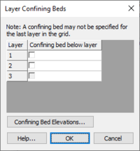
The Layer Confining Beds dialog, accessed from the Global Options/Basic Package dialog, allows selecting which layers will have a confining bed below them. The last layer in the grid may not have a confining bed.
Confining beds are most common in older models where the user was trying to conserve memory in solving the groundwater model. In general, it is recommended that users explicitly model all of the layers in the system instead of using confining beds. This feature is supported in GMS to make it possible for users to read in older models.
In the spreadsheet, the user may turn on the confining bed option for any of the layers except the last layer in the grid.
The Confining Bed Elevations button brings up the Array Editor that allows the user to edit the elevation of each layer.
| GMS – Groundwater Modeling System | ||
|---|---|---|
| Modules: | 2D Grid • 2D Mesh • 2D Scatter Point • 3D Grid • 3D Mesh • 3D Scatter Point • Boreholes • GIS • Map • Solid • TINs • UGrids | |
| Models: | FEFLOW • FEMWATER • HydroGeoSphere • MODAEM • MODFLOW • MODPATH • mod-PATH3DU • MT3DMS • MT3D-USGS • PEST • PHT3D • RT3D • SEAM3D • SEAWAT • SEEP2D • T-PROGS • ZONEBUDGET | |
| Aquaveo | ||

