GMS:MF6 CNC Package
| This contains information about functionality available starting at GMS version 10.6. The content may not apply to other versions. |
| MODFLOW 6 is currently in Beta release for GMS Some features and capabilities of MODFLOW 6 are still in development for GMS. |
| MODFLOW 6 | |
|---|---|
| Models & Tools | |
|
GWF Model GWT Model Cell Properties Dialog Zone File | |
| Packages | |
| Flow: | GNC, HFB, NPF |
| GWF: |
BUY, CHD, CSUB, DRN, EVT, GHB, LAK, MAW, MVR, OBS, RCH,RIV, SFR, STO, UZF, WEL |
| GWT: |
ADV, CNC, DSP FMI, IC, IST, LKT, MDT, MST, MVT, MWT, OBS, SFT, SRC,SSM, UZT |
| Other |
DIS, DISU, DISV, IMS, OC, TDIS, PEST |
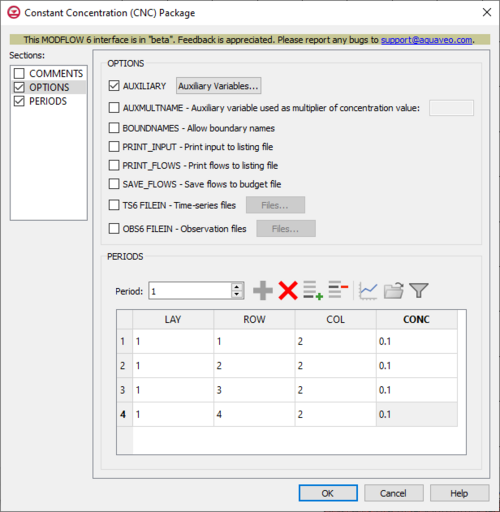
The Constant Concentration (CNC) Package dialog is accessed by double-clicking on the CNC package under a MODFLOW 6 simulation in the Project Explorer. It contains the following sections and options:
- Sections list – A list of sections that can be turned on or off:
- COMMENTS – Turn on to make the COMMENTS section visible.
- OPTIONS – Turn on to make the OPTIONS section visible.
- PERIODS – Turn on to make the PERIODS section visible.
- COMMENTS section – Enter general alphanumeric comments. Comments entered here get written at the top of the file, preceded by a '#' symbol.
- OPTIONS section – Options and settings:
- AUXILIARY – This allows an array of one or more auxiliary variables to be named. There are no limits to the number of auxiliary variables that can be provided, but subsequent blocks will require data for each of the auxiliary variables that are defined. Turning this on will activate an Auxiliary Variables... button. Clicking the button will bring up an Auxiliary Variables dialog.
- AUXMULTNAME – This allows for an auxiliary variable to be used as a multiplier of concentration value. A textbox to the right of the option can be used to specify the name.
- BOUNDNAMES – This indicates that boundary names are allowed to be provided with the list of constant concentration cells. This will add the BOUNDNAME column to the spreadsheet in the PERIODS section.
- PRINT_INPUT – This indicates that the list of constant concentration information input will be printed to the listing file immediately after it is read.
- PRINT_FLOWS – This indicates that the list of constant concentration flow rates will be printed to the listing file. Flow rates will be printed for the last time step of each stress period.
- SAVE_FLOWS – This indicates that constant concentration flow terms will be saved to a budget file (specified in Output Control with "BUDGET FILEOUT").
- TS6 FILEIN – This allows time series files to be used as input to assign time-varying values. Specifying this option will allow a Files... button to its right to be clicked. Doing so will bring up a Files... dialog.
- OBS6 FILEIN – This allows observations files to be used as input. Specifying this option will allow a Files... button to its right to be clicked. Doing so will bring up an Observation Files dialog. In this dialog, a spreadsheet can be filled in that has two columns. The first column allows filenames to be specified. The second column has an Edit... button relating to the file specified. The following options can be used to help develop the spreadsheet:
- Insert Row – This will insert a new row at the current location.
- Add Row – This will add a new row at the bottom.
- Delete Row – This will delete the currently selected row.
- Move Up – This will move the currently selected row up a row.
- Move Down – This will move the currently selected row down a row.
- PERIODS section – This deals with the PERIODS block.
- Period – A numeric updown can be used to enter which period is being examined in the spreadsheet.
- Define Period – This button will allow a period to be defined. This will be active when no period has yet been defined, and it may gray out once one has been created.
- Delete Period – This button will delete the selected period. A dialog warning will come up first asking the user to confirm their decision to delete the period.
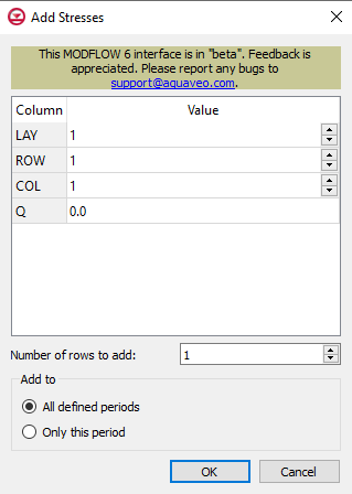
- Add Rows – This button will bring up an Add Stresses dialog. The following options can be used to help in adding the stresses:
- Columns and Values – Numeric updowns and textboxes can be used to enter the values for their relevant columns for all the new stresses. These may include columns that are not actually present in the spreadsheet.
- Number of rows to add – A numeric updown can be used to enter the number of rows that will be added to the spreadsheet.
- Add to – There are two different options, only one of which can be selected at a time.
- All defined periods – These stresses will be added to all the periods that have been defined.
- Only this period – These stresses will be added only to the currently selected period.
- Delete Rows – This button will delete all of the stresses. A dialog warning will come up first asking the user to confirm their decision to delete the stresses. The dialog will also give them the option to either Delete From All Periods or Delete From Just This Period.
- Plot All Periods – This will allow the user to plot all the periods that have been defined.
- Open Time Series – This will allow the user to open a time series file.
- Filter on Selected Cells – ???
- CELLID – This will display differently in the spreadsheet based on what type of grid is used for the simulation, specifically which type of DIS* input file is used in the model. The CELLID is the cell identifier, and the type of DIS* file used will change what will be determined to be the CELLID.
- For a structured grid that uses a DIS input file, these columns will be:
- LAY – This column represents the layers of the cells.
- ROW – This column represents the rows of the cells.
- COL – This column represents the columns of the cells.
- For a grid that uses a DISV input file, these columns will be:
- LAY – This column represents the layers of the cells.
- CELL2D – This column represents the CELL2D numbers of the cells.
- If the model uses a DISU (unstructured discretization) file, the column will be:
- CELLID – This column represents the node numbers of the cells.
- For a structured grid that uses a DIS input file, these columns will be:
- CONC – This column represents the constant concentration values. If time series files are used as input, entering a time series name instead of a numeric value can allow for values to be obtained from a time series.
- AUX – These columns represent the values of the auxiliary variables for each constant concentration, which previously may have been created if the AUXILIARY option was set. If time series files are used as input, entering a time series name instead of a numeric value can allow for values to be obtained from a time series.
- BOUNDNAME – This column represents the names of the constant concentration cells, and will appear if the BOUNDNAMES option was set. BOUNDNAME values are ASCII character variables that can contain as many as 40 characters. If a BOUNDNAME value contains spaces within it, then the entire name will have to be enclosed within single quotes.
Contents
Auxiliary Variables Dialog
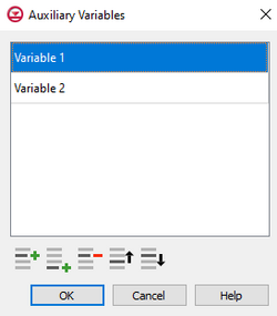
The Auxiliary Variables dialog is accessed by clicking Auxiliary Variables... in the Options section of many package dialogs. It is used to define an array of one or more auxiliary variable names. It contains the following sections and buttons:
- At the top is an unlabeled section listing all of the variables, one per line. Double-click on a variable name to rename it.
- Insert Row
 – Click to insert a row above the currently-selected row.
 - Add Row
 – Click to add a row below the currently-selected row.
 - Delete Row
 – Click to delete the selected row.
 - Move Up
 – Move the selected row up.
 - Move Down
 – Move the selected row down.
Note that each variable name must be unique. If two or more variables share a name, variables added since opening the dialog will not be saved.
Time Series Files Dialog
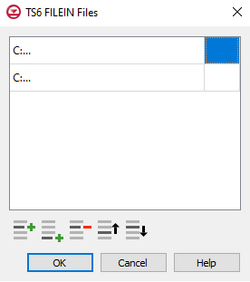
The Time Series Files dialog is accessed by clicking Time Series Files... in the Options section of many of the package dialogs. It is used to define an array of one or more time series files. It contains the following sections and buttons:
- At the top is an unlabeled section listing all of the time series files, one per line.
- Double-click on the first field to see the full file path and name.
- Click Edit... to open the time series file.
- Insert Row
 – Click to insert a row above the currently-selected row.
 - Add Row
 – Click to add a row below the currently-selected row.
 - Delete Row
 – Click to delete the selected row.
 - Move Up
 – Move the selected row up.
 - Move Down
 – Move the selected row down.
Observation Files Dialog
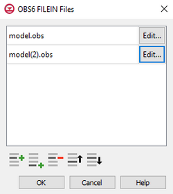
The Observation Files dialog is accessed by clicking Observations... in the Options section of many of the package dialogs. It is used to define an array of one or more observation files. It contains the following sections and buttons:
- At the top is an unlabeled section listing all of the observation files, one per line.
- Double-click on the first field to see the full file path and name.
- Click Edit... to open the Observations (OBS) Dialog.
- Insert Row
 – Click to insert a row above the currently-selected row.
 - Add Row
 – Click to add a row below the currently-selected row.
 - Delete Row
 – Click to delete the selected row.
 - Move Up
 – Move the selected row up.
 - Move Down
 – Move the selected row down.
Add Stresses Dialog
The Add Stresses dialog is accessed by clicking Add Rows ![]() in the Periods section of several MODFLOW 6 package dialogs. It contains the following sections and options:
in the Periods section of several MODFLOW 6 package dialogs. It contains the following sections and options:
- Table – Table Options differ according to each package. See chart below.
- Number of rows to add – Use the Increment Up and Down
 buttons to select the desired number of rows to add.
- Add to section – Radio buttons with the following options:
- All defined periods – Select to add the rows to all defined periods.
- Only this period – Select to add the rows to only this period.
| Package | Add Stresses Dialog Table Options | ||
|---|---|---|---|
| CHD |
| ||
| DRN |
| ||
| GHB |
| ||
| HFB |
| ||
| LAK |
| ||
| MAW |
| ||
| RIV |
| ||
| SFR |
| ||
| UZF |
| ||
| WEL |
|
Related Topics
| GMS – Groundwater Modeling System | ||
|---|---|---|
| Modules: | 2D Grid • 2D Mesh • 2D Scatter Point • 3D Grid • 3D Mesh • 3D Scatter Point • Boreholes • GIS • Map • Solid • TINs • UGrids | |
| Models: | FEFLOW • FEMWATER • HydroGeoSphere • MODAEM • MODFLOW • MODPATH • mod-PATH3DU • MT3DMS • MT3D-USGS • PEST • PHT3D • RT3D • SEAM3D • SEAWAT • SEEP2D • T-PROGS • ZONEBUDGET | |
| Aquaveo | ||
