User:Jcreer/SMS:AdH Interface: Difference between revisions
| (47 intermediate revisions by 2 users not shown) | |||
| Line 306: | Line 306: | ||
=AdH Model Control= | =AdH Model Control= | ||
The ''ADH Model Control'' dialog contains the graphical prompts for specifying model options. The dialog is accessed through the | The ''ADH Model Control'' dialog contains the graphical prompts for specifying model options. The dialog is accessed through right-clicking on the AdH simulation and selecting the '''Model Control...''' item. | ||
The dialog is divided into several tabs which each contain a number of parameter options. Before [[SMS:ADH Run Model|running ADH]], set and review model control parameters. Entered data will be used to write the files employed in the ADH model run. | The dialog is divided into several tabs which each contain a number of parameter options. Before [[SMS:ADH Run Model|running ADH]], set and review model control parameters. Entered data will be used to write the files employed in the ADH model run. | ||
| Line 314: | Line 314: | ||
* ''Time'' – Specifies the simulation duration. By default, ADH uses transient conditions, but steady state simulations can be specified. | * ''Time'' – Specifies the simulation duration. By default, ADH uses transient conditions, but steady state simulations can be specified. | ||
* ''Control Iteration'' – Specifies the level of precision for the conservation of mass and momentum. | * ''Control Iteration'' – Specifies the level of precision for the conservation of mass and momentum. | ||
* ''Control Operation'' – | * ''Control Operation'' – Specifies the number of processors and precoditioner. | ||
* ''Model Control Output'' – Set parameters for how often solution data will be written. | * ''Model Control Output'' – Set parameters for how often solution data will be written. | ||
* ''Control Constants'' – | * ''Control Constants'' – Contains global parameters that are set over the entire domain. | ||
* ''Hot Start'' – Allows setting initial conditions for the simulation. | * ''Hot Start'' – Allows setting initial conditions for the simulation. | ||
* ''Interface'' – Allows maintaining options which are not otherwise supported by the SMS interface. | * ''Interface'' – Allows maintaining options which are not otherwise supported by the SMS interface. | ||
| Line 332: | Line 332: | ||
''Time'' tab provides the following: | ''Time'' tab provides the following: | ||
* ''Start'' time | * ''Start time field'' – Input the start time for the simulation. | ||
* ''Start time units'' | * ''Start time units''– Numbered as seconds, minutes, hours, days, or weeks. | ||
* ''End'' | * ''End time'' – Field (with the defined start) specifies the simulation run length on the <font color="green">TC TF</font> card. | ||
* ''End time units'' | * ''End time units'' – Numbered as seconds, minutes, hours, days, and weeks. | ||
* ''Time step option'' | * ''Time step option'' – Lists one of three options: | ||
** | ** "Steady state solution (TC STD)" | ||
*** ''Steady state min time step size'' | *** ''Steady state min time step size'' – The lowest the time step size should go. | ||
*** ''Steady state max time step size'' | *** ''Steady state max time step size'' – The highest the time step size should go. | ||
** | ** "Time step series (SERIES DT)" | ||
*** Max | *** ''Max Time Series size time differences'' – Clicking the '''Edit Series''' pulls up the ''XY Series Editor''. | ||
** | ** "Auto Time Step Find (TC ATF)" | ||
*** Auto time step find min time step size | *** ''Auto time step find min time step size'' | ||
*** Auto time step find max time step size series | *** ''Auto time step find max time step size series'' | ||
{{-}} | {{-}} | ||
| Line 361: | Line 359: | ||
At the end of each iteration ADH computes the conservation properties for the current approximations of water depth and velocity. If the errors are less than specified tolerance, the solver moves on to the next time step. If the errors are greater than the specified tolerance, but still reasonable, and the maximum number of iterations specified on the IP NIT card has not been reached, ADH will attempt another iteration. If the errors have become unreasonable (divergence), ADH will exit the loop with a failure notification. The controls in this dialog allow defining how ADH should determine convergence and how to proceed when convergence is not reached. | At the end of each iteration ADH computes the conservation properties for the current approximations of water depth and velocity. If the errors are less than specified tolerance, the solver moves on to the next time step. If the errors are greater than the specified tolerance, but still reasonable, and the maximum number of iterations specified on the IP NIT card has not been reached, ADH will attempt another iteration. If the errors have become unreasonable (divergence), ADH will exit the loop with a failure notification. The controls in this dialog allow defining how ADH should determine convergence and how to proceed when convergence is not reached. | ||
*Non Linear Iterations | *''Non Linear Iterations'' – In this edit field specify the maximum number of iterations that ADH will try for a single time step | ||
*''Non Linear Tolerance Options'' | |||
** "NTL (IP_NTL Card)" – If the "NTL" option is selected, ADH will check for non-linear convergence on the "maximum residual norm". An initial estimate for an appropriate tolerance value for a problem can be computed. This is the maximum allowance. It will likely be desirable to set the tolerance higher than this estimate so the simulation will progress. | |||
** "ITL (IP_ITL Card)" – If the ''ITL'' option is selected, ADH will check for non-linear convergence on the "maximum increment norm" or the change in the solution (velocity, depth and concentration). | |||
** "Both" – If the ''Both'' option is selected, SMS will write both cards to the BC file and ADH will check for convergence on both terms. Both must be satisfied for the solution to proceed. | |||
*Non Linear Tolerance | *''Non Linear Residual Tolerance'' – Allows for a solution for residual non-linear iterations. | ||
*''Non Linear Incremental Tolerance'' – Allows for a solution for incremental tolerance iterations. | |||
* | *''Linear Iterations'' – used to solve a linear system of equations when using multiple processors. | ||
* | |||
{{-}} | {{-}} | ||
| Line 376: | Line 373: | ||
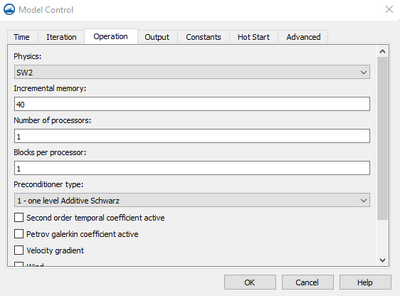
==Operation== | ==Operation== | ||
[[File:ADH Model Operation Control.png|thumb|400 px| ''Operation'' tab of the ''ADH Model Control'' dialog]] | [[File:ADH Model Operation Control.png|thumb|400 px| ''Operation'' tab of the ''ADH Model Control'' dialog]] | ||
*Physics | *''Physics'' | ||
** SW2 | ** "SW2" – used to specify 2D shallow water flow modeling. | ||
** SW3 | ** "SW3" – used to specify 3D shallow water flow modeling | ||
Incremental Memory | *''Incremental Memory'' | ||
Number of Processors | *''Number of Processors'' | ||
Blocks per Processor | *''Blocks per Processor'' | ||
*Preconditioner type | *''Preconditioner type'' – Offers four different options: | ||
**0 | **"0 – none" | ||
**1 One level additive Schwartz | **"1 – One level additive Schwartz" | ||
**2 Two level additive Schwartz | **"2 – Two level additive Schwartz" | ||
**3 Two level hybrid | **"3 – Two level hybrid" | ||
* ''Second order temporal coefficient active'' – Reduces numerical dissipation, higher order temporal schemes are often advantageous for problems where wave reflection is important. | |||
* ''Petrov Galerkin coefficient active'' – can be included in the boundary condition file. | |||
* ''Velocity gradient'' – will preform velocity gradient simulations. | |||
* ''Wind'' – can be included at a single point, or several points, or through a wind field. | |||
* ''Wave'' – when selected will perform wind simulations. | |||
* ''Dam'' – when selected will perform dam break simulations. | |||
{{-}} | {{-}} | ||
==Output== | ==Output== | ||
[[File:ADH Model Output Control.png|thumb|400 px| ''Output'' tab of the ''ADH Model Control'' dialog]] | [[File:ADH Model Output Control.png|thumb|400 px| ''Output'' tab of the ''ADH Model Control'' dialog]] | ||
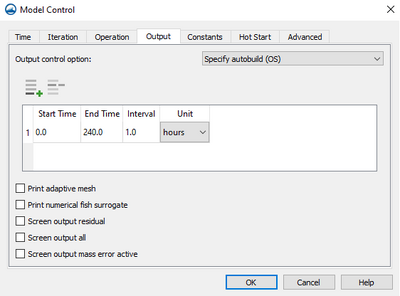
ADH output files are specified in the [[SMS:ADH Model Control|''ADH Model Control'']] dialog | ADH output files are specified in the [[SMS:ADH Model Control|''ADH Model Control'']] dialog on the ''Output'' tab | ||
ADH will write solution data at startup and at each time step specified in a <font color="green">XY1</font> series definition and referred to by the <font color="green">OC</font> card. Flux data will be included with the solution data if output flow strings are specified (see [[ SMS:ADH Boundary Condition Assignment |assigning boundary conditions]]). | ADH will write solution data at startup and at each time step specified in a <font color="green">XY1</font> series definition and referred to by the <font color="green">OC</font> card. Flux data will be included with the solution data if output flow strings are specified (see [[ SMS:ADH Boundary Condition Assignment |assigning boundary conditions]]). | ||
| Line 409: | Line 404: | ||
** "Specify Autobuild (OS)" | ** "Specify Autobuild (OS)" | ||
** "Specify Output Frequency (OC)" | ** "Specify Output Frequency (OC)" | ||
** "Output Control Units" This dropdown lets you choose seconds, minutes, hours, days, and weeks. | ** "Output Control Units" – This dropdown lets you choose seconds, minutes, hours, days, and weeks. | ||
*'''Output Time''' Combo box specifies the time unit the list box will display the output times in. | *'''Output Time''' – Combo box specifies the time unit the list box will display the output times in. | ||
*'''Add [[File:GMS MODFLOW 6 - Add Row button.png]]''' | *'''Add [[File:GMS MODFLOW 6 - Add Row button.png|16 px]]''' – includes the time information from the above radio group in the times list box. Duplicate times will be automatically removed from the list. | ||
*'''Delete [[File:GMS MODFLOW 6 - Delete Rows button.png]]''' | *'''Delete [[File:GMS MODFLOW 6 - Delete Rows button.png|16 px]]''' – removes the selected time(s) from the list box. | ||
*''Print adaptive mesh'' | *''Print adaptive mesh'' – prints the mesh. | ||
*''Print numerical fish surrogate'' | *''Print numerical fish surrogate'' – will print TecPlot format of the numerical fish surrogate. | ||
*''Screen Output Residual'' | *''Screen Output Residual'' – generates a portion of data that may not be explained in the model. | ||
*''Screen Output All'' | *''Screen Output All'' – This puts all the screen output out. | ||
*''Screen Output Mass Error Active'' | *''Screen Output Mass Error Active'' – This makes the mass error output active. | ||
| Line 425: | Line 420: | ||
==Constants== | ==Constants== | ||
[[File:ADH Model Constants Control.png|thumb|400 px| ''Constants'' tab of the ''ADH Model Control'' dialog]] | [[File:ADH Model Constants Control.png|thumb|400 px| ''Constants'' tab of the ''ADH Model Control'' dialog]] | ||
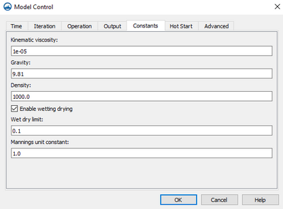
The ''Constants'' tab contains global parameters that are set over the entire domain. global | The ''Constants'' tab contains global parameters that are set over the entire domain. These parameters will be global constants and independent of spatial variations within the model. | ||
*''Kinematic Viscosity'' – Enter a postive real number for the kinematic viscosity. | *''Kinematic Viscosity'' – Enter a postive real number for the kinematic viscosity. | ||
*''Uniform background viscosity'' – Enter a positive real number for background viscosity. | *''Uniform background viscosity'' – Enter a positive real number for background viscosity. | ||
*''Gravitation acceleration'' – Enter a positive real number for gravitation acceleration. | *''Gravitation acceleration'' – Enter a positive real number for gravitation acceleration. | ||
*''Density'' – Enter a positive real number for density. | *''Density'' – Enter a positive real number for density. | ||
*Enable Wetting/drying' is check box and the associated wetting and drying process. When this toggle is selected, AdH performs extra calculations for all cells with depth values less than the specified minimum to stabilize the process. As the specified depth value increases, extra calculations also increase and model performance decreases. | *''Enable Wetting/drying'' – is check box and the associated wetting and drying process. When this toggle is selected, AdH performs extra calculations for all cells with depth values less than the specified minimum to stabilize the process. As the specified depth value increases, extra calculations also increase and model performance decreases. | ||
**''Wet dry limit'' – ADH will decide the wet dry limit. | |||
*''Mannings unit constant'' – Calculates changes in the model | |||
{{-}} | {{-}} | ||
| Line 457: | Line 453: | ||
[[File:ADH Model Advanced Control.png|thumb|400 px| ''Advanced'' tab of the ''ADH Model Control'' dialog]] | [[File:ADH Model Advanced Control.png|thumb|400 px| ''Advanced'' tab of the ''ADH Model Control'' dialog]] | ||
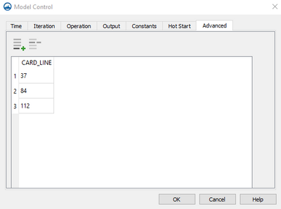
Model options not available in the interface can be specified under the ''Advanced'' tab. Each row in the spreadsheet will be saved as a different line in the *.bc file. The cards can be inserted and deleted using the '''Insert Row''' [[File:Insert Row Icon.svg|16 px]] and '''Delete Row''' [[File:Delete Row Icon.svg|16 px]] buttons. | Model options not available in the interface can be specified under the ''Advanced'' tab. Each row in the spreadsheet will be saved as a different line in the *.bc file. The cards can be inserted and deleted using the '''Insert Row''' [[File:Insert Row Icon.svg|16 px]] and '''Delete Row''' [[File:Delete Row Icon.svg|16 px]] buttons. | ||
*'''Add [[File:GMS MODFLOW 6 - Add Row button.png|16 px]]''' – button includes the information in the Card_Line. | |||
*'''Delete [[File:GMS MODFLOW 6 - Delete Rows button.png|16 px]]''' – button removes the selected time(s) from the list box. | |||
* The lines will be written out exactly as typed. | * The lines will be written out exactly as typed. | ||
* The lines will be written out in the order in which they appear in the dialog. | * The lines will be written out in the order in which they appear in the dialog. | ||
| Line 463: | Line 461: | ||
* Comment lines are automatically generated and will not be preserved. | * Comment lines are automatically generated and will not be preserved. | ||
* All of these advanced cards will be grouped together at the bottom of the file regardless of where they appeared during reading. | * All of these advanced cards will be grouped together at the bottom of the file regardless of where they appeared during reading. | ||
{{-}} | {{-}} | ||
==Related Topics== | ==Related Topics== | ||
*[[SMS:ADH Model Control | ADH Model Control]] | *[[SMS:ADH Model Control | ADH Model Control]] | ||
=AdH Project Workflow= | |||
This is a top level workflow. This workflow includes all of the specific workflows users will need to use in creating an [[SMS:ADH|ADH]] project. Newer and infrequent SMS users should start here. | |||
To build an ADH model in SMS, use the following steps: | |||
{| class="mw-collapsible mw-collapsed" style="width:80%; border:1px solid #D0E0FF; margin-bottom:0.4em;" | |||
|- | |||
!style="text-align:left;"|1. Start a new SMS project. | |||
|- | |||
| | |||
<blockquote> | |||
{{SMS Project Setup Workflow}} | |||
</blockquote> | |||
|} | |||
{|class="mw-collapsible mw-collapsed" style="width:80%; border:1px solid #D0E0FF; margin-bottom:0.4em;" | |||
|- | |||
!style="text-align:left;"|2. Import data. | |||
|- | |||
| | |||
<blockquote> | |||
{{SMS Import Data Workflow}} | |||
</blockquote> | |||
|} | |||
{|class="mw-collapsible mw-collapsed" style="width:80%; border:1px solid #D0E0FF; margin-bottom:0.4em;" | |||
|- | |||
!style="text-align:left;"|3. Review and edit the elevation data. | |||
|- | |||
| | |||
<blockquote> | |||
{{SMS Review-Edit Elevation Data Workflow}} | |||
</blockquote> | |||
|} | |||
{|class="mw-collapsible mw-collapsed" style="width:80%; border:1px solid #D0E0FF; margin-bottom:0.4em;" | |||
|- | |||
!style="text-align:left;"|4. Define model limits (domain extents). | |||
|- | |||
| | |||
<blockquote> | |||
{{SRH Define Model Limits Workflow}} | |||
</blockquote>> | |||
|} | |||
{|class="mw-collapsible mw-collapsed" style="width:80%; border:1px solid #D0E0FF; margin-bottom:0.4em;" | |||
|- | |||
! style="text-align:left;"|5. Generate a mesh. | |||
|- | |||
| | |||
<blockquote> | |||
{{SRH Generate Mesh Workflow}} | |||
</blockquote> | |||
|} | |||
{|class="mw-collapsible mw-collapsed" style="width:80%; border:1px solid #D0E0FF; margin-bottom:0.4em;" | |||
|- | |||
!style="text-align:left;"|6. Define materials for AdH. | |||
|- | |||
| | |||
<blockquote> | |||
{{ADH Materials Workflow}} | |||
</blockquote> | |||
|} | |||
{|class="mw-collapsible mw-collapsed" style="width:80%; border:1px solid #D0E0FF; margin-bottom:0.4em;" | |||
|- | |||
! style="text-align:left;"|7. Define boundary conditions. | |||
|- | |||
| | |||
<blockquote> | |||
{{ADH Boundary Conditions Workflow}} | |||
</blockquote> | |||
|} | |||
{|class="mw-collapsible mw-collapsed" style="width:80%; border:1px solid #D0E0FF; margin-bottom:0.4em;" | |||
|- | |||
!style="text-align:left;"|8. Create the AdH Simulation. | |||
|- | |||
| | |||
<blockquote> | |||
{{AdH Simulation Workflow}} | |||
</blockquote> | |||
|} | |||
{|class="mw-collapsible mw-collapsed" style="width:80%; border:1px solid #D0E0FF; margin-bottom:0.4em;" | |||
|- | |||
!style="text-align:left;"|9. Define the AdH model parameters. | |||
|- | |||
| | |||
:# Right-click on the [[SMS:AdH Simulations|simulation]] and select the '''Model Control''' command. | |||
:# Set the model parameters in the [[SMS:AdH Model Control|AdH ''Model Control'']] dialog. | |||
|} | |||
{|class="mw-collapsible mw-collapsed" style="width:80%; border:1px solid #D0E0FF; margin-bottom:0.4em;" | |||
|- | |||
!style="text-align:left;"|10. Run the AdH Simulation. | |||
|- | |||
| | |||
:# Right-click on the AdH simulation and select '''Save Project, Simulation and Run''']to run the simulation. | |||
:#*Use the [[SMS:Simulations#Simulation_Run_Queue|''Simulation Run Queue'']] to track the model run. | |||
|} | |||
{|class="mw-collapsible mw-collapsed" style="width:80%; border:1px solid #D0E0FF; margin-bottom:0.4em;" | |||
|- | |||
!style="text-align:left;"|11. Review results. | |||
|- | |||
| | |||
<blockquote> | |||
{{SMS Review Results Workflow}} | |||
</blockquote> | |||
|} | |||
Latest revision as of 21:52, 17 October 2023
AdH Coverages
The AdH interface includes a few map coverages. These map coverages are used to provide input for the AdH simulation. AdH use the following model specific coverages:
- Boundary Conditions
- Materials
- Sediment Materials
AdH Boundary Conditions
ADH boundary conditions consist of two specification types (Dirichlet and Natural) and three condition types (flow, pressure, and transport). Dirichlet data is applied on the domain to individual nodes or to groups of nodes (defined with nodestrings). Natural data (flux) is applied through edges of the domain defined by nodestrings and includes a friction specification. A node or nodestring can be assigned only one condition option from each of the three condition types (two flow conditions cannot be assigned to a single node).
The boundary conditions coverage for AdH allows assigning boundary condition attributes for both arcs and points.
Arc Attributes
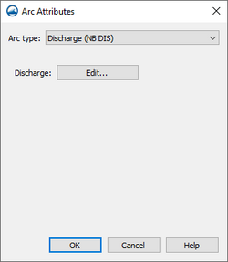
The Arc Attributes dialog is reached by right-clicking on an arc in the AdH boundary conditions and selecting the Assign Arc Attributes command. In the dialog, the Arc type option have several boundary condition attributes for the selected arc. The following Arc type options are as follows:
- "Off" – No attributes will be assigned to the arc.
- "Natural outflow (OB OF)" – allows flow out without any modification to flow properties. Can be specified on boundaries where the exact flow conditions are unknown.
- "Discharge (NB DIS)" – Applies subcritical inflow as a natural total discharge boundary condition.
- Discharge – Clicking Edit opens the XY Series Editor dialog where discharge values can be entered.
- "Flow (NB OVL)" – Applies inflow as a natural unit discharge boundary condition.
- Flow per unit area – Clicking Edit opens the XY Series Editor dialog where discharge values can be entered.
- "Water surface elevation (NB OTW)" – Links a particular time series of water surface elevation to the boundary condition.
- Elevation – Clicking Edit opens the XY Series Editor dialog where water surface elevation values can be entered.
- "Spillway (NB SPL)" – Specifies spillway flow.
- % flow out – Clicking Edit opens the XY Series Editor dialog where weir coefficient values can be entered.
- "Tidal boundary (NB TID)" – Indicates tidal constituents will be applied to the boundary.
- "Stage discharge boundary (NB SDR)" – Specifies a stage-discharge boundary.
- Coefficient – Specified constants for coefficients A–E.
- "Velocity and depth (DB OVH)" – Dirichlet boundary condition for supercritical flow.
- Snapping type – Defines how the boundary conditions are applied to mesh.
- "Point snap" – Applies the attributes to the mesh nodes or points upon export.
- "Edgestring snap" – Applies the attributes to the mesh element edge upon export.
- "Midstring snap" – Applies the attributes to the center of the mesh elements upon export.
- X velocity – Clicking Edit opens the XY Series Editor dialog where x-velocity values can be entered.
- Y velocity – Clicking Edit opens the XY Series Editor dialog where y-velocity values can be entered.
- Depth – Clicking Edit opens the XY Series Editor dialog where depth values can be entered.
- Snapping type – Defines how the boundary conditions are applied to mesh.
- "Stationary lid elevation (DB LDE)" – Allows assigning lid elevations to an arc.
- Snapping type
- Point snap
- Edgestring snap
- Midstring snap
- Elevation – Clicking Edit opens the XY Series Editor dialog where elevation values can be entered.
- Snapping type
- "Depth of water under stationary lid (DB LDH)" – Allows assigning lid depths to an arc.
- Snapping type
- Point snap
- Edgestring snap
- Midstring snap
- Depth – Clicking Edit opens the XY Series Editor dialog where depth values can be entered.
- Snapping type
- "Floating stationary object (DB LID)" – Allows assigning liddraft to an arc.
- Snapping type
- Point snap
- Edgestring snap
- Midstring snap
- Draft of lid – Clicking Edit opens the XY Series Editor dialog where draft values can be entered.
- Snapping type
Arc Friction
Friction controls are used to compute estimated values of the friction induced by several types of bed roughness and linear roughness conditions.
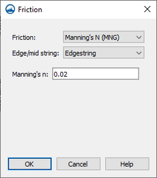
Friction can be applied to a feature arc by right-clicking on the arc and selecting the Assign Friction command. In the Friction dialog, specify the Friction type as one of the following options:
- "Off" – No friction will be applied to the arc.
- "Manning's N (MNG)" – Friction will be applied using Manning's n.
- Edge/mid string
- Edgestring
- Midstring
- Manning's n – Specify the value of Manning's n.
- Edge/mid string
- "Manning's Equation (MNC)" – Friction will be applied using the classic formulation Manning's n.
- Edge/mid string
- Edgestring
- Midstring
- Manning's n – Specify the value of Manning's n.
- Edge/mid string
- "Equivalent roughness height (ERH)" – Friction will be applied using equivalent sand roughness height.
- Edge/mid string
- Edgestring
- Midstring
- Roughness height – Enter a value for the equivalent sand roughness height.
- Edge/mid string
- "Submerged aquatic vegetation (SAV)" – Compute the drag coefficient associated with the bottom shear stress resulting from a steady current field over a bed consisting of submerged aquatic vegetation.
- Edge/mid string
- Edgestring
- Midstring
- Roughness height of canopy – Enter a value for the roughness height of the SAV canopy.
- Undeflected stem height – Enter a value for the undeflected stem height of the SAV.
- Edge/mid string
- "Un-submerged rigid vegetation (URV)" – Compute a shear stress coefficient for use in computing the bottom shear stress resulting from a steady current through rigid, unsubmerged vegetation.
- Edge/mid string
- Edgestring
- Midstring
- Bed roughness height – Enter a value for the bed roughness height.
- Average stem diameter – Enter a value for the average stem diameter.
- Average stem density – Enter a value for the average stem density.
- Edge/mid string
- "Equivalent drag obstructions (EDO)" – Computes a shear stress coefficient for use in computing the shear stress resulting from a steady current through or over an evenly distributed field of flow obstructions.
- Edge/mid string
- Edgestring
- Midstring
- Bed roughness height – Enter a value for the bed roughness height.
- Obstruction diameter – Enter a value for the average obstruction diameter.
- Obstruction height – Enter a value for the average obstruction height.
- Edge/mid string
- "Ice friction (ICE, IRH, BRH)" – Applies as a pressure field on the water surface to account for the effects that stationary ice on the water surface has on the flow below.
- Edge/mid string
- Edgestring
- Midstring
- Ice thickness
- Ice density – Enter a value for the density of ice.
- Ice movement
- Ice roughness height – Enter a value for the equivalent ice roughness height.
- Bed roughness height – Enter a value for the equivalent bed roughness height.
- Edge/mid string
- "Dune friction (DUN)" – Invokes the bedform friction model.
- Edge/mid string
- Edgestring
- Midstring
- Dune factor – Enter a value for the bedform roughness calibration coefficient.
- Dune SEDLIB Inclusion – Turn on to use the sediment model for bedload
- Dune D50 – Enter a value for the d50 of the bed material.
- Dune D90 – Enter a value for the d90 of the bed material.
- Edge/mid string
- "Submerged dike (SDK)" – Simulates the loss associated with the expansion of flow downstream of a submerged dike or weir.
- Dike height – Enter a value for the height of the dike above the bed.
- "Bridge deck (BRD)" – Simulates the the loss associated with a bridge deck.
- Bridge deck elevation – Enter a value for the elevation of the bridge deck.
- Bridge deck thickness – Enter a value for the thickness of the bridge deck.
Flux Output
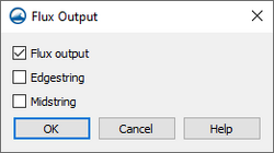
The flux output calculates of flow and constituent mass across strings. To assign flux to a feature arc, right-click on the arc and select the Assign Flux command to open the Flux Output dialog. The Flux Output dialog contains the following options:
- Flux output – Turn on to include fluz output calculations in the model run.
- Edgestring – Select if the flux output is to be calculated along the edge of the mesh domain.
- Midstring – Select if the flux output is to be calculated from internal strings inside the mesh domain.
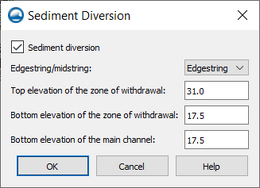
Sediment Diversion
- Sediment diversion – Turn on to include sediment diversion at the feature object location.
- Edgestring/midstring
- "Edgestring"
- "Midstring"
- Top elevation of the zone of withdrawal – Enter the highest elevation for withdrawal area.
- Bottom elevation of the zone of withdrawal – Enter the lowest elevation for withdrawal area.
- Bottom elevation of the main channel – Enter the lowest elevation of the primary channel of the river or stream.
- Edgestring/midstring
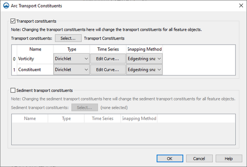
Arc Transport Constituents
The Arc Transport Constituents dialog allows assigning transport constituents to an arc. This requires that transport constituents component to have been created in the AdH simulation. To assign transport constituents to a feature arc, right-click on the arc and select the Assign Arc Transport command to open the Arc Transport Constituents dialog. The Arc Transport Constituents dialog contains the following options:
- Transport constituents – Turning on this option will allow assigning transport constituents.
- Transport constituents – Clicking the Select button will open the Select Transport Constituent dialog where a transport component can be selected. Once the transport component has been selected, the table in this section can be completed.
- Name – This column will display the name of the transport constituents that are active in the Transport Constituents dialog.
- Type – This column allows setting the transport constituent to be "None", "Dirichlet", or "Natural".
- Time Series – This column becomes active if the "Dirichlet" or "Natural" type is selected. Clicking the Edit Curve button will open the XY Series Editor dialog where the time series can be entered.
- Snapping Method
- Transport constituents – Clicking the Select button will open the Select Transport Constituent dialog where a transport component can be selected. Once the transport component has been selected, the table in this section can be completed.
- Sediment transport constituents – Turning on this option will allow assigning sediment transport constituents.
- Sediment transport constituents – Clicking the Select button will open the Select Sediment Transport Constituent dialog where a transport component can be selected. Once the transport component has been selected, the table in this section can be completed.
- Name – This column will display the name of the transport constituents that are active in the Sediment Transport Constituents dialog.
- Type – This column allows setting the transport constituent to be "None", "Dirichlet", or "Natural".
- Time Series – This column becomes active if the "Dirichlet" or "Natural" type is selected. Clicking the Edit Curve button will open the XY Series Editor dialog where the time series can be entered.
- Snapping Method
- Sediment transport constituents – Clicking the Select button will open the Select Sediment Transport Constituent dialog where a transport component can be selected. Once the transport component has been selected, the table in this section can be completed.
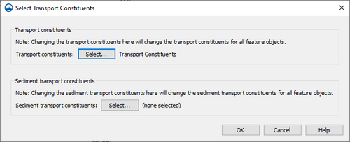
Select Transport Constituents
When working with transport constituents, the transport constituent component in the simulation needs be attached to transport constituents attributes assigned to feature objects. In the Project Explorer, right-clicking on the AdH boundary condition coverage and selecting the Assign Transport command will being up the Select Transport Constituents dialog. This dialog allows assigning the transport feature object attributes to the transport components.
- Transport constituents – Clicking the Select button in this section will being up the Select Transport Constituents dialog. In the Select Transport Constituents dialog, the transport component can be assigned to the coverage.
- Sediment transport constituents – Clicking the Select button in this section will being up the Select Sediment Transport Constituents dialog. In the Select Sediment Transport Constituents dialog, the transport component can be assigned to the coverage.
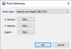
Point Attributes
The Point Attributes dialog is reached by right-clicking on a point in the AdH boundary conditions and selecting the Assign Point Attributes command. In the dialog, the Point type option have several boundary condition attributes for the selected point. The following Point type options are as follows:
- "Off" – No attributes will be assigned to the point.
- "Velocity and depth (DB OVH)" – Dirichlet boundary condition for supercritical flow.
- X velocity – Clicking Edit opens the XY Series Editor dialog where x-velocity values can be entered.
- Y velocity – Clicking Edit opens the XY Series Editor dialog where y-velocity values can be entered.
- Depth – Clicking Edit opens the XY Series Editor dialog where depth values can be entered.
- "Stationary lid elevation (DB LDE)" – Allows assigning lid elevations to an arc.
- Elevation – Clicking Edit opens the XY Series Editor dialog where elevation values can be entered.
- "Depth of water under stationary lid (DB LDH)" – Allows assigning lid depths to an arc.
- Depth – Clicking Edit opens the XY Series Editor dialog where depth values can be entered.
- "Floating stationary object (DB LID)" – Allows assigning liddraft to an arc.
- Draft of lid – Clicking Edit opens the XY Series Editor dialog where draft values can be entered.
- "Wind Definition (OP WND)" – Defines wind stressing.
- Wind – Clicking Edit opens the XY Series Editor dialog where wind values can be entered.
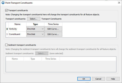
Point Transport Constituents
The Point Transport Constituents dialog allows assigning transport constituents to a point. This requires that transport constituents component to have been created in the AdH simulation. To assign transport constituents to a feature point, right-click on the point and select the Assign Point Transport command to open the Point Transport Constituents dialog. The Popint Transport Constituents dialog contains the following options:
- Transport constituents – Turning on this option will allow assigning transport constituents.
- Transport constituents – Clicking the Select button will open the Select Transport Constituent dialog where a transport component can be selected. Once the transport component has been selected, the table in this section can be completed.
- Name – This column will display the name of the transport constituents that are active in the Transport Constituents dialog.
- Type – This column allows setting the transport constituent to be "None" or "Dirichlet".
- Time Series – This column becomes active if the "Dirichlet" type is selected. Clicking the Edit Curve button will open the XY Series Editor dialog where the time series can be entered.
- Transport constituents – Clicking the Select button will open the Select Transport Constituent dialog where a transport component can be selected. Once the transport component has been selected, the table in this section can be completed.
- Sediment transport constituents – Turning on this option will allow assigning sediment transport constituents.
- Sediment transport constituents – Clicking the Select button will open the Select Sediment Transport Constituent dialog where a transport component can be selected. Once the transport component has been selected, the table in this section can be completed.
- Name – This column will display the name of the transport constituents that are active in the Sediment Transport Constituents dialog.
- Type – This column allows setting the transport constituent to be "None" or "Dirichlet".
- Time Series – This column becomes active if the "Dirichlet" type is selected. Clicking the Edit Curve button will open the XY Series Editor dialog where the time series can be entered.
- Sediment transport constituents – Clicking the Select button will open the Select Sediment Transport Constituent dialog where a transport component can be selected. Once the transport component has been selected, the table in this section can be completed.
AdH Materials
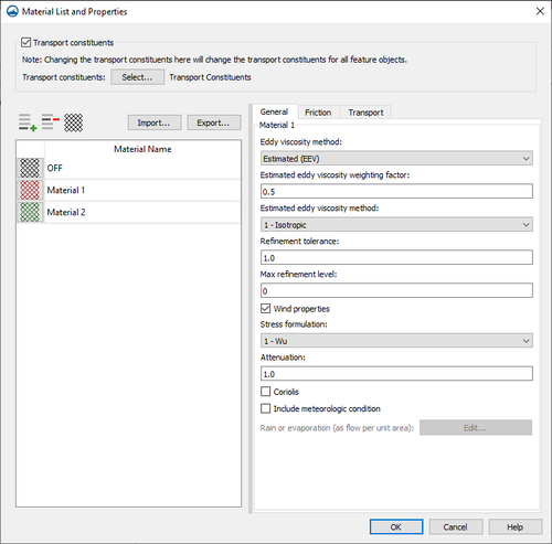
Material properties are set for AdH on an AdH materials coverage. In the Project Explorer, define the material attributes by right-clicking the materials coverage and selecting Material List and Properties to open the Material List and Properties dialog. The Material List and Properties dialog contains the following options:
- Transport constituents – Turning on this option will allow assigning transport constituents.
- Transport constituents – Clicking the Select button will open the Select Transport Constituent dialog where a transport component can be selected.
- Add Rows
 – Adds a material item to the list below this.
 - Delete Rows
 – Removes a selected material.
 - Change all material textures
 – Brings up the Texture Attributes dialog where the texture for all materials can be changed.
 - Import – Brings up an Open dialog where an AdH material file (*.adh_mat) can be imported into the dialog.
- Export – Brings up a Save dialog where an AdH materila file (*adh_mat) can be exported.
- Material list – The Materials list contains two columns (Color and Name) for the defined materials. The default "OFF" material cannot be edited (except the display pattern) and will always be at the top of the spreadsheet regardless of sorting. Each material is accompanied by a Color button in the Color column. To select a color and pattern, click on the button to open the Texture Attributes window. On the right side of the dialog, the numeric properties of the material are displayed and can be edited.
General
The General tab of the AdH Material List and Properties dialog contains the following options:
- Eddy viscosity method – Defines the eddy viscosity for the simulation using one of two methods. Both methods cannot be used for
one material, but both can be used in a single model.
- "Estimated (EEV)" – Defines eddy viscosity utilizing an equation to estimate the value.
- Estimated eddy viscosity weighing factor – Enter a value for the weighting factor.
- Estimated eddy viscosity method – Select one of the following methods:
- "1 – Isotropic"
- "2 – Anisotropic"
- "3 – Smagorinsky"
- "4 – Stansby"
- "Constant (EVS)" – Defines eddy viscosity through a user specified constant value.
- Vxx eddy viscosity
- Vxy eddy viscosity
- Vyy eddy viscosity
- "Estimated (EEV)" – Defines eddy viscosity utilizing an equation to estimate the value.
- Refinement tolerance – Enter a value to refine and relax the resolution of the model mesh during the simulation run.
- Max refinement level – Enter a value for the maximum level of mesh refinement.
- Wind properties – Check on to include wind stress calculations.
- Stress formulation – Select the method that will be used for wind stress.
- "0 – no transform"
- "1 – Wu"
- "2 – Teeter"
- Attenuation – Enter a scale factor to increase or decrease the wind shear stress magnitude.
- Stress formulation – Select the method that will be used for wind stress.
- Coriolis – Turn on to include the Coriolis force due to the earth’s rotation.
- Coriolis latitude – Enter a value for the latitude in decimal degrees.
- Include meteorologic condition – Turn on to include rain or evaporation for the material.
- Rain or evaporation – Click the Edit button to open an XY Series Editor dialog where rainfall or evaporation data can be entered.
Friction
- Friction
- "Off" – No friction will be applied to the model.
- "Manning's n (MNG)" – Friction will be applied using Manning's n.
- Manning's n – Specify the value of Manning's n.
- "Manning's Equation (MNC)" – Friction will be applied using the classic formulation Manning's n.
- Manning's n – Specify the value of Manning's n.
- "Equivalent roughness height (ERH)" – Friction will be applied using equivalent sand roughness height.
- Roughness height – Enter a value for the equivalent sand roughness height.
- "Submerged aquatic vegetation (SAV)" – Compute the drag coefficient associated with the bottom shear stress resulting from a steady current field over a bed consisting of submerged aquatic vegetation.
- Roughness height of canopy – Enter a value for the roughness height of the SAV canopy.
- Undeflected stem height – Enter a value for the undeflected stem height of the SAV.
- "Un-submerged rigid vegetation (URV)" – Compute a shear stress coefficient for use in computing the bottom shear stress resulting from a steady current through rigid, unsubmerged vegetation.
- Bed roughness height – Enter a value for the bed roughness height.
- Average stem diameter – Enter a value for the average stem diameter.
- Average stem density – Enter a value for the average stem density.
- "Equivalent drag obstructions (EDO)" – Computes a shear stress coefficient for use in computing the shear stress resulting from a steady current through or over an evenly distributed field of flow obstructions.
- Bed roughness height – Enter a value for the bed roughness height.
- Obstruction diameter – Enter a value for the average obstruction diameter.
- Obstruction height – Enter a value for the average obstruction height.
- "Ice friction (ICE, IRH, BRH)" – Applies as a pressure field on the water surface to account for the effects that stationary ice on the water surface has on the flow below.
- Ice thickness
- Ice density – Enter a value for the density of ice.
- Ice movement
- Ice roughness height – Enter a value for the equivalent ice roughness height.
- Bed roughness height – Enter a value for the equivalent bed roughness height.
- "Dune friction (DUN)" – Enter a value for the bedform roughness calibration coefficient.
- Dune Factor –
- Dune SEDLIB Inclusion – Turn on to use the sediment model for bedload
- Dune D50 – Enter a value for the d50 of the bed material.
- Dune D90 – Enter a value for the d90 of the bed material.
- Include Seasonal Roughness Adjustment
- Roughness adjustment factor
Transport
The Transport tab allows adjusting the tolerance for transport constituents going through the material. The tab requires that a transport constituent component to be selected.
AdH Sediment Materials
AdH Simulation
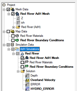
Simulations are available for AdH starting in SMS 13.3. A simulation should contain a 2D mesh and an AdH boundary conditions coverage, and optional AdH coverages. Right-clicking on the simulation will display options and dialogs.
To create a new simulation:
- Right-click on empty space in the Project Explorer and select New Simulation | AdH. A new tree item
 will appear.
 - Drag and drop simulation components under the newly created simulation tree item
 . Components available include:
- 2D mesh
- Boundary Conditions coverage
- Materials coverage
Multiple AdH simulations can be included in a single project.
Simulation Components
An AdH simulation uses the following components in the model run:
- 2D mesh – Any generic 2D mesh will work. Generally this mesh should be created from the Mesh Generation coverage.
- Boundary Conditions coverage – Contains arcs defining the boundary condition attributes for the model run.
- Materials coverage – Allows creating recording stations at specified nodal locations.
- Sediment Material coverage –
Each component can be added to the simulation by selecting the component and dragging it under the simulation item ![]() in the Project Explorer. Linked 2D mesh
in the Project Explorer. Linked 2D mesh ![]() and coverages
and coverages ![]() will be displayed under the simulation.
will be displayed under the simulation.
Linking Components
After a simulation has been created, components may be added to the simulation. Components are usually added by clicking on the component item in the Project Explorer and dragging the item under the AdH simulation. A link ![]() is then created between the component and the simulation.
is then created between the component and the simulation.
Components can also be added to a simulation by right-clicking on the component in the project explorer and selecting the simulation name in the Apply To submenu. The Apply To submenu becomes available once a simulation has been created.
Components can be removed by right-clicking on the component link under the simulation and select Remove.
If a component is updated, it must be reapplied to the simulation.
Running the AdH Simulation
After all components have been added to the simulation and the model parameters have been established, the simulation can be run. This is done by right-clicking on the simulation and choosing the Run Simulation command or the Save and Run Simulation command.
The simulation run involves three steps.
- Exporting the AdH files – SMS writes out an AdH folder in the same directory where the SMS project is saved. The AdH folder has several files which have mesh geometry information, and boundary conditions as well as model control information defined in the model.
- Running AdH – After using a launch command, the Simulation Run Queue dialog will appear. If there are any errors in the model run, the model wrapper will exit early. The model run can also be exited early by clicking the Abort button. When the model run is completed, select Exit to close the model wrapper.
The Load solution button appears with the model run has finished. Clicking this button will load the solution into SMS.
AdH Model Control
The ADH Model Control dialog contains the graphical prompts for specifying model options. The dialog is accessed through right-clicking on the AdH simulation and selecting the Model Control... item.
The dialog is divided into several tabs which each contain a number of parameter options. Before running ADH, set and review model control parameters. Entered data will be used to write the files employed in the ADH model run.
The available tabs are:
- Time – Specifies the simulation duration. By default, ADH uses transient conditions, but steady state simulations can be specified.
- Control Iteration – Specifies the level of precision for the conservation of mass and momentum.
- Control Operation – Specifies the number of processors and precoditioner.
- Model Control Output – Set parameters for how often solution data will be written.
- Control Constants – Contains global parameters that are set over the entire domain.
- Hot Start – Allows setting initial conditions for the simulation.
- Interface – Allows maintaining options which are not otherwise supported by the SMS interface.
See the individual articles for each of the ADH model control tabs.
Time
DH is set up as a transient conditions model, however, a steady state simulation can be invoked which utilizes an iterative process to converge to a solution. A steady state solution is accepted if the end time of the model is reached or the iteration tolerance requirement (see Model Parameters ) is met. It's required to ensure that all series data are acceptable (constant linear series) if the steady state method is used. ADH also includes a quasi-unsteady method which strings multiple steady state simulation together to form a step function style hydrograph.
Due to the nature of a steady state simulation, constituent transport and bed layers cannot be included in the simulation. If any constituent (and bed layer) is specified in a dynamic simulation and then the simulation is changed to steady state, SMS will clear the constituent data (and bed layer specification). A message will warn of this effect when the steady state simulation type is selected and constituent data (and a bed layer) exists. Another message will state that SMS has cleared the data (if steady state is still selected) when switching to another tab or exiting Model Control by selecting OK.
Since series data specified for a dynamic simulation is usually inappropriate for a steady state simulation, a change in simulation type from dynamic to steady state will force SMS to clear all previously specified series data when changes are accepted in Model Control. This data is usually associated with the boundary conditions of materials, nodes, and nodestrings. A message will warn of this effect when the simulation type is changed and series data exists. Another message will state that SMS has cleared the data (if the simulation type remains changed) upon accepting the changes (exiting Model Control).
The following controls specify the timing parameters for the ADH model run.
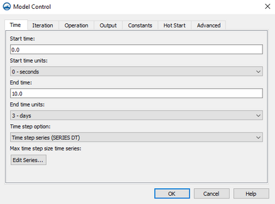
Time tab provides the following:
- Start time field – Input the start time for the simulation.
- Start time units– Numbered as seconds, minutes, hours, days, or weeks.
- End time – Field (with the defined start) specifies the simulation run length on the TC TF card.
- End time units – Numbered as seconds, minutes, hours, days, and weeks.
- Time step option – Lists one of three options:
- "Steady state solution (TC STD)"
- Steady state min time step size – The lowest the time step size should go.
- Steady state max time step size – The highest the time step size should go.
- "Time step series (SERIES DT)"
- Max Time Series size time differences – Clicking the Edit Series pulls up the XY Series Editor.
- "Auto Time Step Find (TC ATF)"
- Auto time step find min time step size
- Auto time step find max time step size series
- "Steady state solution (TC STD)"
Iteration
The Iterations tab allows specifying the level of precision for the conservation of mass and momentum as ADH performs its calculations.
ADH solves conservation statements concerning water volume, momentum, and constituent mass. ADH is written in conservative form and thus can be regarded as both a finite element method and also a finite volume method. As such ADH can be shown to represent a sum of fluxes around the edge of an element to be in balance with the mass or volume change within the element. In the case of the momentum equation it will be a sum of fluxes and forces balancing the momentum change within an element.
ADH computes the water levels and velocities at each computation point in the domain for each time step in the simulation in an iterative process. At the end of each iteration, calculations are made to determine how much the solution is changing and what the errors in conservation are. If the errors are small, and the solution is not changing, the process is said to be converged and calculations can proceed to the next time step. If the solution is changing and/or the errors in conservation are large, ADH can attempt another iteration.
There are several iteration parameter controls in ADH. These are described in detail in the ADH users manual. The Advanced options tab controls the linear iterations. This dialog controls the non-linear iteration parameters.
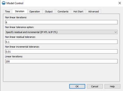
At the end of each iteration ADH computes the conservation properties for the current approximations of water depth and velocity. If the errors are less than specified tolerance, the solver moves on to the next time step. If the errors are greater than the specified tolerance, but still reasonable, and the maximum number of iterations specified on the IP NIT card has not been reached, ADH will attempt another iteration. If the errors have become unreasonable (divergence), ADH will exit the loop with a failure notification. The controls in this dialog allow defining how ADH should determine convergence and how to proceed when convergence is not reached.
- Non Linear Iterations – In this edit field specify the maximum number of iterations that ADH will try for a single time step
- Non Linear Tolerance Options
- "NTL (IP_NTL Card)" – If the "NTL" option is selected, ADH will check for non-linear convergence on the "maximum residual norm". An initial estimate for an appropriate tolerance value for a problem can be computed. This is the maximum allowance. It will likely be desirable to set the tolerance higher than this estimate so the simulation will progress.
- "ITL (IP_ITL Card)" – If the ITL option is selected, ADH will check for non-linear convergence on the "maximum increment norm" or the change in the solution (velocity, depth and concentration).
- "Both" – If the Both option is selected, SMS will write both cards to the BC file and ADH will check for convergence on both terms. Both must be satisfied for the solution to proceed.
- Non Linear Residual Tolerance – Allows for a solution for residual non-linear iterations.
- Non Linear Incremental Tolerance – Allows for a solution for incremental tolerance iterations.
- Linear Iterations – used to solve a linear system of equations when using multiple processors.
Operation
- Physics
- "SW2" – used to specify 2D shallow water flow modeling.
- "SW3" – used to specify 3D shallow water flow modeling
- Incremental Memory
- Number of Processors
- Blocks per Processor
- Preconditioner type – Offers four different options:
- "0 – none"
- "1 – One level additive Schwartz"
- "2 – Two level additive Schwartz"
- "3 – Two level hybrid"
- Second order temporal coefficient active – Reduces numerical dissipation, higher order temporal schemes are often advantageous for problems where wave reflection is important.
- Petrov Galerkin coefficient active – can be included in the boundary condition file.
- Velocity gradient – will preform velocity gradient simulations.
- Wind – can be included at a single point, or several points, or through a wind field.
- Wave – when selected will perform wind simulations.
- Dam – when selected will perform dam break simulations.
Output
ADH output files are specified in the ADH Model Control dialog on the Output tab
ADH will write solution data at startup and at each time step specified in a XY1 series definition and referred to by the OC card. Flux data will be included with the solution data if output flow strings are specified (see assigning boundary conditions).
The following controls specify how often solution data will be written by ADH and the number of flux boundaries present.
- Output Control Options:
- "Specify Autobuild (OS)"
- "Specify Output Frequency (OC)"
- "Output Control Units" – This dropdown lets you choose seconds, minutes, hours, days, and weeks.
- Output Time – Combo box specifies the time unit the list box will display the output times in.
- Add
 – includes the time information from the above radio group in the times list box. Duplicate times will be automatically removed from the list.
 - Delete
 – removes the selected time(s) from the list box.
 - Print adaptive mesh – prints the mesh.
- Print numerical fish surrogate – will print TecPlot format of the numerical fish surrogate.
- Screen Output Residual – generates a portion of data that may not be explained in the model.
- Screen Output All – This puts all the screen output out.
- Screen Output Mass Error Active – This makes the mass error output active.
Constants
The Constants tab contains global parameters that are set over the entire domain. These parameters will be global constants and independent of spatial variations within the model.
- Kinematic Viscosity – Enter a postive real number for the kinematic viscosity.
- Uniform background viscosity – Enter a positive real number for background viscosity.
- Gravitation acceleration – Enter a positive real number for gravitation acceleration.
- Density – Enter a positive real number for density.
- Enable Wetting/drying – is check box and the associated wetting and drying process. When this toggle is selected, AdH performs extra calculations for all cells with depth values less than the specified minimum to stabilize the process. As the specified depth value increases, extra calculations also increase and model performance decreases.
- Wet dry limit – ADH will decide the wet dry limit.
- Mannings unit constant – Calculates changes in the model
Hot Start
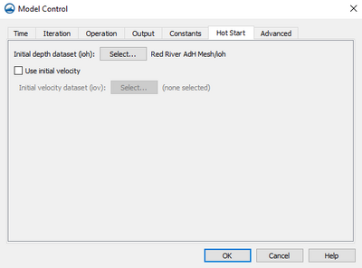
The hot start file contains the initial conditions for each node of a mesh. ADH allows for the specification of depth and velocity hydrodynamics, and sediment concentration and displacement datasets. The model requires at least depth initial conditions for hydrodynamics, and non-specified conditions.
- Initial depth dataset (ioh) – Clicking the Select button here will bring up the Select initial depth dataset dialog. The initial depth dataset will be used for the initial depth at the start of the simulation.
- Use Initial Velocity – Turn on the include initial velocity in the simulation.
- Initial velocity dataset (iov) – Clicking the Select button will bring up the Select initial velocity dataset dialog. The initial velocity dataset will be used for the initial velocity at the start of the simulation.
Advanced
AdH features not supported by SMS can be added in the ADH Model Control dialog by clicking on the Advanced tab.
SMS includes support for many of the features in ADH, however, this list of features is a dynamic set. The user base of ADH includes a development team that is constantly experimenting with new options.
This window allows SMS to maintain the options that are not otherwise supported by the interface. For example, when SMS reads the BC file for an ADH simulation, and encounters a card that it does not recognize, that card is stored, verbatim, to a list of "Advanced Cards". That list is displayed in this window.
Enter cards in this dialog to experiment with other new features in the model. As those features are added to the list of supported features, they would automatically be moved to their own location in the model control the next time SMS reads the BC file.
Unsupported or advanced cards are written at the end of the BC file, just before the END card. This relies on the attribute of ADH that does not require any order dependence in the BC file.
Model options not available in the interface can be specified under the Advanced tab. Each row in the spreadsheet will be saved as a different line in the *.bc file. The cards can be inserted and deleted using the Insert Row ![]() and Delete Row
and Delete Row ![]() buttons.
buttons.
- Add
 – button includes the information in the Card_Line.
 - Delete
 – button removes the selected time(s) from the list box.
 - The lines will be written out exactly as typed.
- The lines will be written out in the order in which they appear in the dialog.
- Any lines encountered in a *.bc file that is not recognized will appear in this list.
- Lines beginning with a "!" character are treated as comment lines and will be skipped over during a read.
- Comment lines are automatically generated and will not be preserved.
- All of these advanced cards will be grouped together at the bottom of the file regardless of where they appeared during reading.
Related Topics
AdH Project Workflow
This is a top level workflow. This workflow includes all of the specific workflows users will need to use in creating an ADH project. Newer and infrequent SMS users should start here.
To build an ADH model in SMS, use the following steps:
| 1. Start a new SMS project. | ||||
|---|---|---|---|---|
|
| 2. Import data. | ||||||||||||||||||||||
|---|---|---|---|---|---|---|---|---|---|---|---|---|---|---|---|---|---|---|---|---|---|---|
|
| 3. Review and edit the elevation data. | ||||||||||||||||||
|---|---|---|---|---|---|---|---|---|---|---|---|---|---|---|---|---|---|---|
|
| 4. Define model limits (domain extents). | ||||||||||||||||||||||||||||||||||||||||||||||||||||
|---|---|---|---|---|---|---|---|---|---|---|---|---|---|---|---|---|---|---|---|---|---|---|---|---|---|---|---|---|---|---|---|---|---|---|---|---|---|---|---|---|---|---|---|---|---|---|---|---|---|---|---|---|
> |
| 5. Generate a mesh. | ||||||||||||||||||||||||||||||||||||||||||||
|---|---|---|---|---|---|---|---|---|---|---|---|---|---|---|---|---|---|---|---|---|---|---|---|---|---|---|---|---|---|---|---|---|---|---|---|---|---|---|---|---|---|---|---|---|
|
| 6. Define materials for AdH. | ||||||||||||||||||||||||||||||||||||||||||
|---|---|---|---|---|---|---|---|---|---|---|---|---|---|---|---|---|---|---|---|---|---|---|---|---|---|---|---|---|---|---|---|---|---|---|---|---|---|---|---|---|---|---|
|
| 7. Define boundary conditions. | ||||||||||||||||||||||||||||||||||||||
|---|---|---|---|---|---|---|---|---|---|---|---|---|---|---|---|---|---|---|---|---|---|---|---|---|---|---|---|---|---|---|---|---|---|---|---|---|---|---|
|
| 8. Create the AdH Simulation. | ||||
|---|---|---|---|---|
|
| 9. Define the AdH model parameters. |
|---|
|
| 10. Run the AdH Simulation. |
|---|
|
| 11. Review results. | ||||||||||||||||||||||||||||||||||||||||||||||||||||||||||||||||||||||||||||||||||||||||||||||||||||||||||
|---|---|---|---|---|---|---|---|---|---|---|---|---|---|---|---|---|---|---|---|---|---|---|---|---|---|---|---|---|---|---|---|---|---|---|---|---|---|---|---|---|---|---|---|---|---|---|---|---|---|---|---|---|---|---|---|---|---|---|---|---|---|---|---|---|---|---|---|---|---|---|---|---|---|---|---|---|---|---|---|---|---|---|---|---|---|---|---|---|---|---|---|---|---|---|---|---|---|---|---|---|---|---|---|---|---|---|
|
SMS – Surface-water Modeling System | ||
|---|---|---|
| Modules: | 1D Grid • Cartesian Grid • Curvilinear Grid • GIS • Map • Mesh • Particle • Quadtree • Raster • Scatter • UGrid |  |
| General Models: | 3D Structure • FVCOM • Generic • PTM | |
| Coastal Models: | ADCIRC • BOUSS-2D • CGWAVE • CMS-Flow • CMS-Wave • GenCade • STWAVE • WAM | |
| Riverine/Estuarine Models: | AdH • HEC-RAS • HYDRO AS-2D • RMA2 • RMA4 • SRH-2D • TUFLOW • TUFLOW FV | |
| Aquaveo • SMS Tutorials • SMS Workflows | ||
