GMS:MODFLOW Conceptual Model Approach: Difference between revisions
From XMS Wiki
Jump to navigationJump to search
| (24 intermediate revisions by 5 users not shown) | |||
| Line 4: | Line 4: | ||
== Definition == | == Definition == | ||
In GMS, the term conceptual model is used in two different ways. In the generic sense, a conceptual model is a simplified representation of the site to be modeled including the model domain, boundary conditions | In GMS, the term conceptual model is used in two different ways. In the generic sense, a conceptual model is a simplified representation of the site to be modeled including the model domain, boundary conditions (BCs), and material zones. GMS also has a conceptual model object, that can be defined in the [[GMS:Map Module|Map module]]. The conceptual model object can contain coverages. | ||
A conceptual model object can be defined in the [[GMS:Map Module|Map module]] using [[GMS:Feature Objects|feature objects]], such as points, arcs, and polygons. The conceptual model is constructed <u>independently</u> of the numerical grid. Once the conceptual model object is defined, a grid can be automatically generated to fit the conceptual model. The boundary conditions and model parameters are computed and assigned to the proper cells. The MODFLOW data are converted from the conceptual model to the cells of the grid. This approach to modeling fully automates the majority of the data entry and eliminates the need for most or all of the tedious cell-by-cell editing traditionally associated with MODFLOW modeling. Once the conceptual model is constructed and [[GMS:Map to MODFLOW|converted to a grid]], the package dialogs and interactive editing tools in the MODFLOW menu can be used to edit or review the data if desired. | A conceptual model object can be defined in the [[GMS:Map Module|Map module]] using [[GMS:Feature Objects|feature objects]], such as points, arcs, and polygons. The conceptual model is constructed ''<u>independently</u>'' of the numerical grid. Once the conceptual model object is defined, a grid can be automatically generated to fit the conceptual model. The boundary conditions and model parameters are computed and assigned to the proper cells. The MODFLOW data are converted from the conceptual model to the cells of the grid. This approach to modeling fully automates the majority of the data entry and eliminates the need for most or all of the tedious cell-by-cell editing traditionally associated with MODFLOW modeling. Once the conceptual model is constructed and [[GMS:Map to MODFLOW|converted to a grid]], the package dialogs and interactive editing tools in the ''MODFLOW'' menu can be used to edit or review the data if desired. | ||
A complete conceptual model object consists of several coverages. One coverage is typically used to define the sources and sinks such as wells, rivers, lakes, and drains. Another coverage (or the same coverage) is used to define the recharge zones. Other coverages can be used to define the zones of hydraulic conductivity within each layer. Any number of coverages may be used, or all these attributes may exist in the same coverage. | A complete conceptual model object consists of several coverages. One coverage is typically used to define the sources and sinks such as wells, rivers, lakes, and drains. Another coverage (or the same coverage) is used to define the recharge zones. Other coverages can be used to define the zones of hydraulic conductivity within each layer. Any number of coverages may be used, or all these attributes may exist in the same coverage. | ||
| Line 13: | Line 13: | ||
== Steps in Developing a Conceptual Model == | == Steps in Developing a Conceptual Model == | ||
Several steps are involved in setting up a | Several steps are involved in setting up a MODFLOW conceptual model and converting the conceptual model to a numerical model. The basic steps are as follows: | ||
#Create a MODFLOW conceptual model in the Map | #Create a MODFLOW conceptual model in the Map module. | ||
#Decide how many coverages | #Decide how many coverages are needed and what attributes are wanted with each. It is typical to use three coverages, each with a different purpose. One coverage is used for sources and sinks, like wells, specified head boundaries etc. Another coverage is used for recharge, and another is used for hydraulic conductivity. However, it is not required to use coverages in this manner, and the attributes associated with a coverage are user defined, so define a coverage with any combination of attributes. Thus, if the recharge zones were the same as the hydraulic conductivity zones, it is possible to use just one coverage for both. | ||
#Create the sources and sinks. The most effective way to do this is with the aid of a background [[GMS:Images|Image]]. A digital image representing a scanned map or an aerial photo of the site can be imported and displayed in the background using the image tools. Once the image is displayed, [[GMS:Feature Objects|feature objects]] defining the model boundary, rivers, lakes, flow barriers, and specified head boundaries can be created on top of the background image. | #Create the sources and sinks. The most effective way to do this is with the aid of a background [[GMS:Images|Image]]. A digital image representing a scanned map or an aerial photo of the site can be imported and displayed in the background using the image tools. Once the image is displayed, [[GMS:Feature Objects|feature objects]] defining the model boundary, rivers, lakes, flow barriers, and specified head boundaries can be created on top of the background image. | ||
#Create the areal features, such as recharge zones and evapotranspiration zones. | #Create the areal features, such as recharge zones and evapotranspiration zones. | ||
#Create the layer features, such as hydraulic conductivity zones. | #Create the layer features, such as hydraulic conductivity zones. | ||
#Use the [[GMS:Grid Frame| | #Use the [[GMS:Grid Frame|'''Grid Frame''']] command to place an outline of the numerical grid on the conceptual model. The frame is placed so that it just surrounds the conceptual model. The frame can be rotated if necessary if the major axis of the model is at an angle. | ||
#Use the ''Feature Objects | Map | #Use the ''Feature Objects'' | '''Map → 3D Grid''' command to automatically generate a grid. The location of the grid is controlled by the Grid Frame and the density of the grid is automatically adjusted around user-specified points (typically wells). | ||
#Define the active region of the grid using the [[GMS:Activate Cells in Coverage|Activate Cells in Coverage]] command. This automatically activates all of the cells within the boundary of the conceptual model and inactivates all cells outside the boundary. | #Define the active region of the grid using the [[GMS:Activate Cells in Coverage|'''Activate Cells in Coverage''']] command. This automatically activates all of the cells within the boundary of the conceptual model and inactivates all cells outside the boundary. | ||
#Initialize the MODFLOW data by selecting the | #Initialize the MODFLOW data by selecting the '''New Simulation''' command in the ''MODFLOW'' menu. Select the type of mode (steady state vs. transient) and define [[GMS:Stress Periods|stress periods]] if necessary. Define a set of starting heads. Go to the ''LPF/BCF/HUF Package'' dialog and define the layer type for each of the layers in the grid. | ||
#Select the [[GMS:Map to MODFLOW| | #Select the [[GMS:Map to MODFLOW|'''Map → MODFLOW''']] command to automatically assign the MODFLOW boundary conditions, stresses, and material properties to the appropriate cells in the grid. | ||
#Use the [[GMS:Defining | #Use the [[GMS:Defining Layer Elevations|specialized interpolation]] tools to define the layer elevations. | ||
In many cases, it is useful to repeat some, but not all, of these steps. For example, suppose after running a simulation it is determined that one of the boundaries of the model corresponding to a groundwater divide is not properly located. The boundary can be moved by simply selecting and dragging the vertices and nodes of the arc(s) defining the boundary. Once the boundary is moved, step 6 should be repeated to redefine the active/inactive regions and then step 8 is repeated to reassign the model data to the cells. | In many cases, it is useful to repeat some, but not all, of these steps. For example, suppose after running a simulation it is determined that one of the boundaries of the model corresponding to a groundwater divide is not properly located. The boundary can be moved by simply selecting and dragging the vertices and nodes of the arc(s) defining the boundary. Once the boundary is moved, step 6 should be repeated to redefine the active/inactive regions and then step 8 is repeated to reassign the model data to the cells. | ||
== Example Application == | == Example Application == | ||
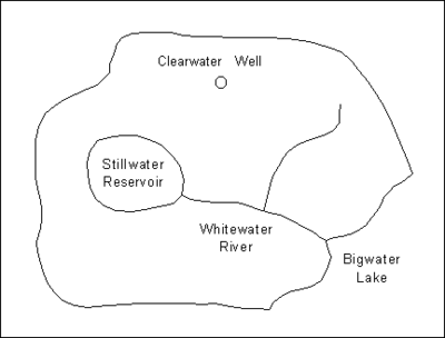
To illustrate the conceptual model approach, consider the site shown in the following figure. It represents information that might be available from a combination of sources including maps, photos, and GIS data. This information may include the location of hydrologic features as well as hydrologic properties of the site. However, this information is not yet organized into a form that is useful to a numerical model. | To illustrate the conceptual model approach, consider the site shown in the following figure. It represents information that might be available from a combination of sources including maps, photos, and GIS data. This information may include the location of hydrologic features as well as hydrologic properties of the site. However, this information is not yet organized into a form that is useful to a numerical model. | ||
[[Image:sitemap.png|400 px]] | |||
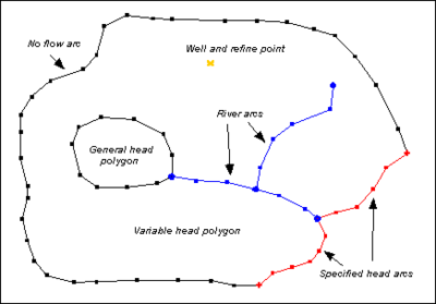
The first step in creating a conceptual model of this site is to create points, arcs and polygons that represent hydrologic features at the site. These points, arcs and polygons are assigned types that correspond to the feature they represent. Based on the attribute type, parameters such as head, concentration and conductance are assigned to these feature objects. The resulting coverage is shown in the following figure. Other coverages, defining such things as recharge zones, would also be defined. | The first step in creating a conceptual model of this site is to create points, arcs and polygons that represent hydrologic features at the site. These points, arcs and polygons are assigned types that correspond to the feature they represent. Based on the attribute type, parameters such as head, concentration and conductance are assigned to these feature objects. The resulting coverage is shown in the following figure. Other coverages, defining such things as recharge zones, would also be defined. | ||
[[Image:concmod.png|400 px]] | |||
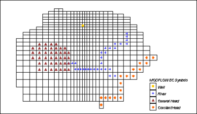
The final step is to take the information that is stored in the conceptual model and construct a numerical model. GMS automates both the creation of the grid geometry as well as assigning boundary conditions and material parameters to the grid. Refine points can be used to specify areas where the grid should have a high density. By specifying polygons that represent the domain of the model, it is possible to automatically inactivate all the cells that lie outside that domain. Boundary conditions may be applied to the individual cells that are intersected by specified feature objects. In addition to determining which cells are assigned boundary conditions, GMS also calculates the appropriate values to assign to each stress period of a transient simulation. The resulting numerical model is illustrated in the following figure. | The final step is to take the information that is stored in the conceptual model and construct a numerical model. GMS automates both the creation of the grid geometry as well as assigning boundary conditions and material parameters to the grid. Refine points can be used to specify areas where the grid should have a high density. By specifying polygons that represent the domain of the model, it is possible to automatically inactivate all the cells that lie outside that domain. Boundary conditions may be applied to the individual cells that are intersected by specified feature objects. In addition to determining which cells are assigned boundary conditions, GMS also calculates the appropriate values to assign to each stress period of a transient simulation. The resulting numerical model is illustrated in the following figure. | ||
[[Image:gridmod.png|400 px]] | |||
== Advantages of the Conceptual Model Approach == | == Advantages of the Conceptual Model Approach == | ||
| Line 46: | Line 46: | ||
There are numerous benefits to the conceptual model approach. First of all, the model can be defined independently of the grid resolution. The modeler does not need to waste valuable time computing the appropriate conductance to assign to a river cell based on the length of the river reach within the cell. This type of computation is performed automatically. Furthermore, transient parameters such as pumping rates for wells can also be assigned independently of model discretization. Transient parameters are entered as a curve of the stress vs. time. When the conceptual model is converted to the numerical model, the transient values of the stresses are automatically assigned to the appropriate stress periods. Since the conceptual model is defined independently of the spatial and temporal discretization of the numerical model, the conceptual model can be quickly and easily changed and a new numerical model can be generated in seconds. This allows the modeler to evaluate numerous alternative conceptual models in the space of time normally required to evaluate one, resulting in a more accurate and efficient modeling process. | There are numerous benefits to the conceptual model approach. First of all, the model can be defined independently of the grid resolution. The modeler does not need to waste valuable time computing the appropriate conductance to assign to a river cell based on the length of the river reach within the cell. This type of computation is performed automatically. Furthermore, transient parameters such as pumping rates for wells can also be assigned independently of model discretization. Transient parameters are entered as a curve of the stress vs. time. When the conceptual model is converted to the numerical model, the transient values of the stresses are automatically assigned to the appropriate stress periods. Since the conceptual model is defined independently of the spatial and temporal discretization of the numerical model, the conceptual model can be quickly and easily changed and a new numerical model can be generated in seconds. This allows the modeler to evaluate numerous alternative conceptual models in the space of time normally required to evaluate one, resulting in a more accurate and efficient modeling process. | ||
A further advantage of storing attributes with feature objects is that the method of applying the boundary conditions to the grid cells reduces some of the instability that is inherent in finite difference models such as MODFLOW and MT3DMS. When | A further advantage of storing attributes with feature objects is that the method of applying the boundary conditions to the grid cells reduces some of the instability that is inherent in finite difference models such as MODFLOW and MT3DMS. When entering individual values for heads and elevations, entering cell values one cell at a time can be tedious. It is also difficult to determine the correct elevation along a river segment at each cell that it crosses. The temptation is to select small groups of cells in series and apply the same values to all of the cells in the group. This results in an extreme stair-step condition that can slow or even prevent convergence of the numerical solver. By using GMS to interpolate values at locations along a linear boundary condition such as a river, it is insured that there will be no abrupt changes from cell to cell-thus minimizing the stair-step effect. It also produces a model with boundary conditions that more accurately represent real world conditions. | ||
== Defining the Layer Data == | == Defining the Layer Data == | ||
An important part of a MODFLOW model is the definition of the layer data (hydraulic conductivity, layer elevations, leakance, etc.). While both the [[GMS:3D Grid Module|Grid]] and [[GMS:Map Module|Map]] module approaches to constructing a MODFLOW model can be used to define the layer data, both approaches may lead to an overly simplistic definition of the stratigraphy. Layers with spatially varying thicknesses can be handled most effectively using a [[GMS:Defining | An important part of a MODFLOW model is the definition of the layer data (hydraulic conductivity, layer elevations, leakance, etc.). While both the [[GMS:3D Grid Module|Grid]] and [[GMS:Map Module|Map]] module approaches to constructing a MODFLOW model can be used to define the layer data, both approaches may lead to an overly simplistic definition of the stratigraphy. Layers with spatially varying thicknesses can be handled most effectively using a [[GMS:Defining Layer Elevations|special set of layer data tools]] provided in GMS. Solids can also be used to define layer data with the [[GMS:Solids to MODFLOW Command|'''Solids→MODFLOW''']] and [[GMS:Solids to HUF|'''Solids→HUF''']] commands. | ||
==See Also== | |||
*[[GMS:Map to MODFLOW|Map to MODFLOW]] | |||
*[[GMS:Conductance|Conductance]] | |||
| Line 56: | Line 60: | ||
[[Category:Conceptual Model]] | [[Category:Conceptual Model]] | ||
[[Category:MODFLOW]] | [[Category:MODFLOW|Concept]] | ||


